Tutorial 01: Model-Based Spectral Calibration using LEAP¶

This tutorial introduces a model-based spectral calibration approach using the LEAP projector.

To run this notebook, you also need to download and install spekpy

In this tutorial, we will

simulate multi-energy dataset using LEAP projector
- simulate CT scans with specific source, filter, and detector configurations.
- scan multiple materials at different source voltages to generate multi-energy dataset.
model-based spectral calibration
- Step 0: Obtain sample masks and calculate forward matrix.
- Step 1: Configure Spectral Models including source, filters, and detector(scintillator).
- Step 2: Spectral Calibration.

X-ray System Setup¶

Source¶

Type: Reflection
Take-off Angle: 13°
Voltages Used for Scanning:
- 50 kV
- 100 kV
- 150 kV

Filter¶

Material: Aluminum (Al)
Thickness: 3 mm

Detector¶

Material: Cesium Iodide (CsI)
Thickness: 0.33 mm

Samples¶

Shapes: Rods with 0.5 mm radius
Materials:
- Vanadium (V)
- Aluminum (Al)
- Titanium (Ti)
- Magnesium (Mg)
Height: 0.2 mm

CT Geometry¶

Beam Type: Cone Beam
Source-to-Object Distance (SOD): 8 mm
Source-to-Detector Distance (SDD): 15 mm
Detector Specifications:
- Pixel Size: 0.01 mm × 0.01 mm
- Scan Shape: 50 × 512 pixels
Number of Views: 64

[1]:

import numpy as np
import matplotlib.pyplot as plt

max_simkV = 180 # keV
takeoff_angle = 13 # degree
voltage_list = [40, 80, 180] # keV
mas_list = [0.01,0.01,0.01] # Milliampere-seconds

fltr_mat = 'Al' # filter material
fltr_th = 3 # filter thickness in mm

det_mat = 'CsI' # scintillator material
det_density = 4.51 # scintillator density g/cm^3
det_th = 0.33 # scintillator thickness in mm

sample_mats = ['V', 'Al', 'Ti', 'Mg']
sample_radius = 0.5 # sample diameter in mm


ct_info = {
    "Geometry": "Cone",
    "SOD": 8, # mm
    "SDD": 15,# mm
    "psize": [0.01875, 0.01875],  # Width and height in mm
    "rsize": [0.01, 0.01],
    "shape": [50, 512],     # Rows and columns
    "NViews": 64
}

A. Simulate multi-energy dataset using LEAP projector¶

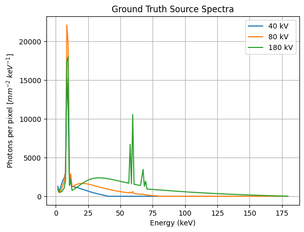
A01. Ground Truth Source Spectra¶

In this tutorial,

use spekpy to generate X-ray source spectum.
the description of 2 used functions from spekpy is shown below by the help function.

[2]:

import spekpy as sp
help(sp.Spek.__init__)

Help on function __init__ in module spekpy.SpekPy:

__init__(self, kvp=None, th=None, dk=None, mu_data_source=None, physics=None, x=None, y=None, z=None, mas=None, brem=None, char=None, obli=None, comment=None, targ=None, shift=None, init_default=True)
    Constructor method for the Spek class

    SEE THE WIKI PAGES FOR MORE INFO:
    https://bitbucket.org/spekpy/spekpy_release/wiki/Further_information

    :param float kvp: tube potential [kV] (default: depends on target)
    :param float th: anode angle [degrees] (default: 12 degrees)
    :param float dk: energy bin width [keV] (default: 0.5 keV)
    :param string: mu_data_source (default: depends on physics model)
        options: ('pene' or 'nist')
    :param float physics: physics model (default: 'casim')
        options: ('casim', 'kqp', 'spekpy-v1', 'spekcalc',
                  'diff', 'uni', 'sim', 'classical')
    :param float x: displacement from central axis in anode-cathode
        direction [cm] (default: 0 cm)
    :param float y: displacement from central axis in orthogonal
        direction [cm] (default: 0 cm)
    :param float z: focus-to-detector distance [cm] (default: 100 cm)
    :param float mas: the tube current-time product [mAs] (default: 1 mAs)
    :param logical brem: whether bremsstrahlung x rays requested
        (default: true)
    :param logical char: whether characteristic x rays requested
        (default: true)
    :param logical obli: whether increased oblique paths through filtration
        are assumed for off axis positions (default: true)
    :param string comment: any text annotation the user wishes to add
    :param string targ: the anode target material (default: 'W')
        options: ('W', 'Mo', or 'Rh')
    :param float shift: optional fraction of an energy bin to shift the
        energy bins (useful when matching to measurements) (default: 0.0)

[3]:

help(sp.Spek.get_spectrum)

Help on function get_spectrum in module spekpy.SpekPy:

get_spectrum(self, edges=False, flu=True, diff=True, sig=None, addend=False, **kwargs)
    A method to get the energy and spectrum for the parameters in the
    current spekpy state

    :param bool edges: Keyword argument to determine whether midbin or edge
        of bins data are returned
    :param bool addend: Keyword argument to determine whether a zero
        end point is added to the spectrum
    :param bool flu: Whether to return fluence or energy-fluence
    :param bool diff: Whether to return spectrum differential in energy
    :param kwargs: Keyword arguments to change parameters that are used for
        the calculation
    :return array k: Array with photon energies (mid-bin or edge values)
        [keV]
    :return array spk: Array with corresponding photon fluences
        [Photons cm^-2 keV^-1], [Photons cm^-2] or [Photons cm^-2 keV^1]
        depending of values of flu and diff inputs

[4]:

max_simkV = max(voltage_list)
takeoff_angle = 13

# Define energy bins from 1.5 keV up to (max_simkV - 0.5) keV.
energies = np.linspace(1.5, max_simkV - 0.5, max_simkV-1)

# Initialize an empty list to store the generated source spectra.
gt_src_spec_list = []

for case_i, simkV in enumerate(voltage_list):
    # Generate the X-ray spectrum model with Spekpy for each voltage.
    # kvp is source voltage
    # th is anode angle
    # dk is energy bin size
    # z is focus-to-detector distance [cm], use source-detector distance instead and convert mm to cm.
    # mas is current-time product mA*s
    # char=True requests characteristic x rays.
    s = sp.Spek(kvp=simkV, th=takeoff_angle, dk=1, z=ct_info['SDD']/10, mas=mas_list[case_i], char=True)

    # Return data at the mid of a bin or the edges of a bin.
    k, phi_k = s.get_spectrum(edges=False)  # Retrieve energy bins and fluence spectrum [Photons cm^-2 keV^-1]

    # Adjust the fluence for the detector pixel area.
    phi_k = phi_k * ((ct_info['psize'][0] / 10) * (ct_info['psize'][1] / 10))  # Convert pixel size from cm² to mm²

    # Initialize a zero-filled spectrum array with length max_simkV.
    src_spec = np.zeros(max_simkV-1)
    src_spec[:simkV-1] = phi_k  # Assign spectrum values starting from 1.5 keV

    # Add the processed spectrum for this voltage to the list.
    gt_src_spec_list.append(src_spec)

# Convert the list of source spectra to a numpy array for easy handling.
gt_src_spec_list = np.array(gt_src_spec_list)

# Plot each generated source spectrum.
for src_i, gt_src_spec in enumerate(gt_src_spec_list):
    plt.plot(energies, gt_src_spec, label='%d kV' % voltage_list[src_i])

plt.title('Ground Truth Source Spectra')
plt.xlabel('Energy (keV)')
plt.ylabel('Photons per pixel [$mm^{-2}$ $keV^{-1}$]')
plt.grid()
plt.legend()

[4]:

<matplotlib.legend.Legend at 0x150b247daf50>

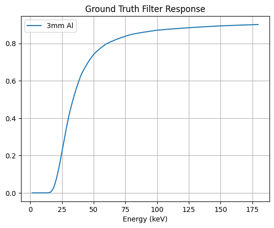
../_images/examples_T01_Calibration_LEAP_7_1.png

A02. Ground Truth Filter Response¶

Filter response is defined as

\[f(E) = e^{-\mu(m, E)\cdot t}\]

where $t$ is thickness; $\mu$ is linear attenuation coefficient(LAC), which depends on photon energy and material $m$ formula and density.

[5]:

from xcal import get_filter_response
from xcal.chem_consts._periodictabledata import density

# get_filter_response returns a ratio of passing through photons.
# F(E) = e^(-\mu_{mat}(E)*thickness)
# \mu_{mat}(E) = mac{mat}(E) * density
# where \mu denotes linear attenuation coefficient; mac means mass attenuation coefficient.
gt_fltr = get_filter_response(energies, fltr_mat, density[fltr_mat], fltr_th)

plt.plot(energies, gt_fltr, label='3mm Al')
plt.title('Ground Truth Filter Response')
plt.legend()
plt.xlabel('Energy (keV)')
plt.grid()

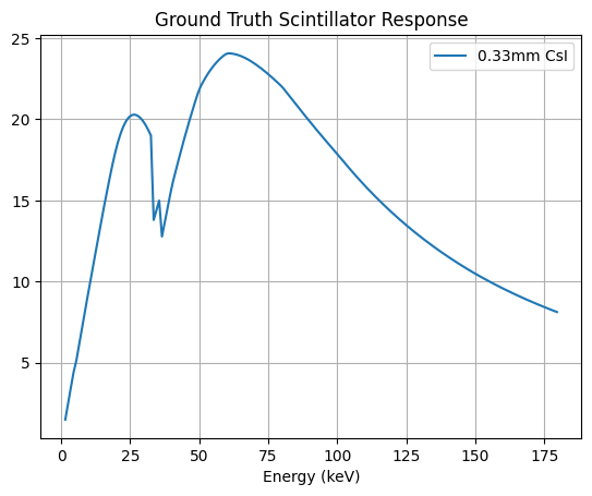
../_images/examples_T01_Calibration_LEAP_9_0.png

A03. Ground Truth Detector Response¶

Converted energy from a X-ray photon with energy from 1 to 180 keV.

Detector response is defined as

\[D(E) =\frac{\mu_{en}(m, E)}{\mu(m, E)} (1 - e^{-\mu(m, E)\cdot t} )\]

where $t$ is scintillator thickness; $\mu$ is linear attenuation coefficient(LAC), which depends on photon energy $E$ and material $m$ formula and density; $\mu_en$ is linear energy-absorption coefficient(LAC).

[6]:

from xcal import get_scintillator_response
from xcal.chem_consts._periodictabledata import density

# get_scintillator_response returns converted energy per photon at energy E.
# D(E) = -\mu_en/\mu * (1-e^(-\mu(E)*thickness))
# \mu(E) = mac(E) * density
# \mu_en(E) = mac_en(E) * density
# where \mu denotes linear attenuation coefficient; mac means mass attenuation coefficient.
# where \mu_en denotes linear energy-absorption coefficient; mac_en means mass energy-absorption coefficient.
gt_det = get_scintillator_response(energies, det_mat, det_density, det_th)

plt.plot(energies, gt_det, label='%.2fmm %s'%(det_th, det_mat))
plt.title('Ground Truth Scintillator Response')
plt.legend()
plt.xlabel('Energy (keV)')
plt.grid()

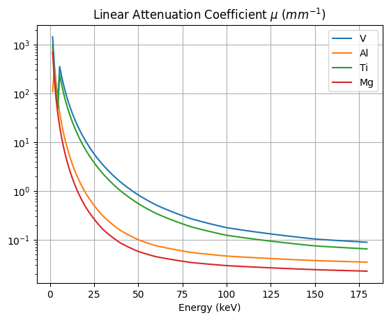
../_images/examples_T01_Calibration_LEAP_11_0.png

A04. Linear Attenuation Coefficients of homogenous samples¶

[7]:

from xcal.chem_consts import get_lin_att_c_vs_E
help(get_lin_att_c_vs_E)

Help on function get_lin_att_c_vs_E in module xcal.chem_consts._consts_from_table:

get_lin_att_c_vs_E(density, formula, energy_vector)
    Calculate the linear attenuation coefficient (mu) as a function of energy,
    using mass attenuation coefficients from the NIST website:
    https://physics.nist.gov/PhysRefData/XrayMassCoef/tab3.html.

    Author: Wenrui Li, Purdue University
    Date: 04/12/2022

    Parameters
    ----------
    density : float
        Density of the material in g/cm^3.
    formula : str/dict
        Chemical formula of the compound, either as a string or a dict.
        For example, "H2O" and {"H": 2, "O": 1} are both acceptable.
    energy_vector : list/numpy.ndarray
        Energy (units: keV) list or 1D array for which beta values are calculated.

    Returns
    -------
    numpy.ndarray
        Linear attenuation coefficient values in mm^-1, with the same size as energy_vector.

[8]:

# Scanned Homogeneous Rods
# Density for homogenous material is stored in the imported density dictionary
mat_density = [density[formula] for formula in sample_mats]
lac_vs_E_list = [get_lin_att_c_vs_E(den, formula, energies) for den, formula in zip(mat_density, sample_mats)]

# Plot LAC
for lac_vs_E,mat in zip(lac_vs_E_list, sample_mats):
    plt.plot(energies, lac_vs_E, label=mat)
plt.yscale('log')
plt.title(r'Linear Attenuation Coefficient $\mu$ ($mm^{-1}$)')
plt.xlabel('Energy (keV)')
plt.grid()
plt.legend()

[8]:

<matplotlib.legend.Legend at 0x150a4f7e9030>

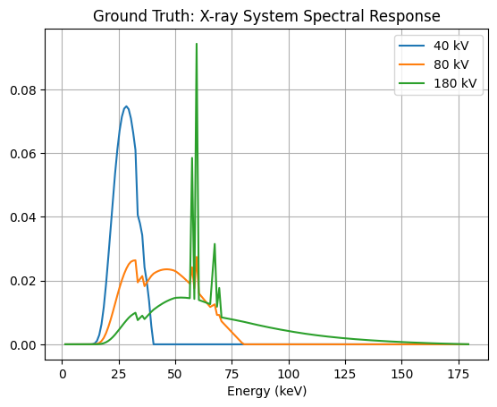
../_images/examples_T01_Calibration_LEAP_14_1.png

A05. GT X-ray System Spectral Responses¶

[9]:

gt_spec_list = [gt_source * gt_fltr  * gt_det for gt_source in gt_src_spec_list]
for spec_i, gt_spec in enumerate(gt_spec_list):
    plt.plot(energies, gt_spec/np.trapezoid(gt_spec,energies), label='%d kV'%voltage_list[spec_i])
plt.legend()
plt.title('Ground Truth: X-ray System Spectral Response')
plt.xlabel('Energy (keV)')
plt.grid()
plt.legend()

[9]:

<matplotlib.legend.Legend at 0x150a4f366260>

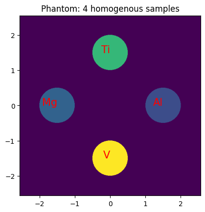
../_images/examples_T01_Calibration_LEAP_16_1.png

A06. Masks for 4 homogenous samples¶

Obtain a list of mask for each corresponding homogenous sample rod. These masks is then used to calculate the forward matrix for the transmission function.

[10]:

from xcal._utils import Gen_Circle
help(Gen_Circle.__init__)

Help on function __init__ in module xcal._utils:

__init__(self, canvas_shape, pixel_size)
    Initialize the Circle class.

    Parameters:
    canvas_shape (tuple): The shape of the canvas, in pixels.
    pixel_size (tuple): The size of a pixel, in the same units as the canvas.

[11]:

help(Gen_Circle.generate_mask)

Help on function generate_mask in module xcal._utils:

generate_mask(self, radius, center=None)
    Generate a binary mask for the circle.

    Parameters:
    radius (int): The radius of the circle, in pixels.
    center (tuple): The center of the circle.

    Returns:
    ndarray: A 2D numpy array where points inside the circle are marked as True and points outside are marked as False.

[12]:

# Define parameters for 4 cylinders with 0.5mm radius, evenly distributed on a circle with a radius of 1.5mm.
Radius = [sample_radius for _ in range(len(sample_mats))]  # Radius of each cylindrical cross-section in mm
arrange_with_radius = 1.5  # Radius of the circle on which cylinder centers are distributed (in mm)

# Calculate center positions for each cylinder, evenly spaced around the circular arrangement
centers = [[np.sin(rad_angle) * arrange_with_radius, np.cos(rad_angle) * arrange_with_radius]
           for rad_angle in np.linspace(-np.pi / 2, -np.pi / 2 + np.pi * 2, len(sample_mats), endpoint=False)]

# Generate 3D masks for each cylinder
# Obtain a list of mask for each corresponding homogenous sample rod.
# These masks is then used to calculate the forward matrix for the transmission function.
mask_list = []
for mat_id, mat in enumerate(sample_mats):
    # Initialize a circular mask generator for 2D slices
    # Use the number of column pixels to define a canvas
    circle = Gen_Circle((ct_info["shape"][1], ct_info["shape"][1]),
                        (ct_info["rsize"][0], ct_info["rsize"][1])) # Image volume size
    # Create a 3D mask array for the current cylinder by repeating the circular 2D mask across slices
    mask_3d = np.array([circle.generate_mask(Radius[mat_id], centers[mat_id])
                        for i in range(ct_info["shape"][0])])
    mask_list.append(mask_3d)

# Below just for display
# Initialize the phantom array to hold combined cylinder masks
phantom = np.zeros(mask_list[0].shape)

# Combine all masks into the phantom, weighted by the linear attenuation coefficients for each material
for mat_id, mat in enumerate(sample_mats):
    phantom += mask_list[mat_id] * np.mean(lac_vs_E_list[mat_id])

# Display a slice of the phantom (e.g., 26th slice) to show cross-sectional circles of cylinders
plt.imshow(phantom[25], extent=[-2.56, 2.56, -2.56, 2.56], origin='lower')

# Annotate each circle with its corresponding material name
for mat_id, mat in enumerate(sample_mats):
    plt.text(centers[mat_id][1], centers[mat_id][0], mat, fontsize=15, ha='right', color='red')
plt.title('Phantom: 4 homogenous samples')

[12]:

Text(0.5, 1.0, 'Phantom: 4 homogenous samples')

../_images/examples_T01_Calibration_LEAP_20_1.png

A07. Setup forward projector with LEAP¶

[13]:

import time
from leapctype import *

class fw_projector:
    """A class for forward projection using LEAP."""

    def __init__(self, numAngles, numRows, numCols, pixelHeight, pixelWidth, centerRow, centerCol, phis, sod, sdd):
        """
        Initializes the forward projector with specified geometric parameters.
        """
        # Initialize parameters as instance variables
        self.numAngles = numAngles
        self.numRows = numRows
        self.numCols = numCols
        self.pixelHeight = pixelHeight
        self.pixelWidth = pixelWidth
        self.centerRow = centerRow
        self.centerCol = centerCol
        self.phis = phis
        self.sod = sod  # Source-to-object distance
        self.sdd = sdd  # Source-to-detector distance
        self.leapct = tomographicModels()
        self.leapct.about()
    def forward(self, mask):
        """
        Computes the projection of a given mask.

        Parameters:
            mask (numpy.ndarray): 3D mask of the object to be projected. 1 for the region of object and 0 elsewhere.

        Returns:
            numpy.ndarray: The computed projection of the mask.
        """

        self.leapct.set_conebeam(self.numAngles,
                            self.numRows,
                            self.numCols,
                            self.pixelHeight,
                            self.pixelWidth,
                            self.centerRow,
                            self.centerCol,
                            self.phis,
                            self.sod,
                            self.sdd)
        self.leapct.set_default_volume()
        proj = self.leapct.allocate_projections() # shape is numAngles, numRows, numCols
        volume = np.ascontiguousarray(mask.astype(np.float32), dtype=np.float32)

        # Obtain projection data
        startTime = time.time()
        self.leapct.project(proj,volume)
        print('Forward Projection Elapsed Time: ' + str(time.time()-startTime))
        return proj

leapct2 = tomographicModels()
projector =fw_projector(ct_info['NViews'],
                        ct_info["shape"][0],
                        ct_info["shape"][1],
                        ct_info["psize"][0],
                        ct_info["psize"][1],
                        0.5*(ct_info["shape"][0]-1),
                        0.5*(ct_info["shape"][1]-1),
                        leapct2.setAngleArray(ct_info['NViews'], 360.0),
                        ct_info["SOD"],
                        ct_info["SDD"])

A08. Calculate Attenuation Matrix¶

We let $ \mu_k(E) $ denote the LAC of the $k^\text{th}$ homogeneous sample at energy $E$, and let $L_{k, i}$ denote the path length through the $k^{th}$ material at projection $i$ for samples $k=0, \ldots, K-1$. The attenuation matrix is calculated as below,

\[A_{i}(E) = \exp \left\{-\sum_{k=0}^{K-1} \mu_k(E) L_{k, i}\right\}\]

Notice that $L_{k, i}$ is calcuated by projecting $k^\text{th}$ mask in mask_list with a projector defined in A07. One should create the “projector” object in a similar way defined in A07 if use CT projector other than LEAP.

[14]:

from xcal import calc_forward_matrix
spec_F = calc_forward_matrix(mask_list, lac_vs_E_list, projector)

Forward Projection Elapsed Time: 0.1924912929534912
Forward Projection Elapsed Time: 0.028488874435424805
Forward Projection Elapsed Time: 0.027208566665649414
Forward Projection Elapsed Time: 0.027233123779296875

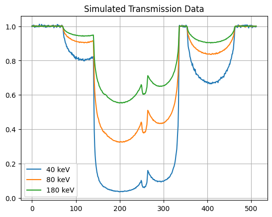
A09. Simulate Transmission Data¶

[15]:

trans_list = []
for case_i, gt_spec in zip(np.arange(len(gt_spec_list)), gt_spec_list):
    # Obtain the converted energy, which is proportional to the detected visible light photons by the camera.
    # gt_spec is the converted energy without an object.
    # Notice that, trapezoid does the energy integration.
    trans = np.trapezoid(spec_F * gt_spec, energies, axis=-1) # Object scan
    trans_0 = np.trapezoid(gt_spec, energies, axis=-1) # Air scan value
    # Add poisson noise.
    # The noise level can be adjusted by changing the mas, the current-time product in the beginning of this tutorial.
    trans_noise = np.random.poisson(trans).astype(np.float32)
    trans_noise /= trans_0

    # Store noisy transmission data.
    trans_list.append(trans_noise)

[16]:

for case_i, gt_spec in enumerate(gt_spec_list):
    plt.plot(trans_list[case_i][3, 25], label=f'{voltage_list[case_i]} keV')
plt.legend()
plt.grid()
plt.title('Simulated Transmission Data')

[16]:

Text(0.5, 1.0, 'Simulated Transmission Data')

../_images/examples_T01_Calibration_LEAP_27_1.png

B. Spectral Calibration¶

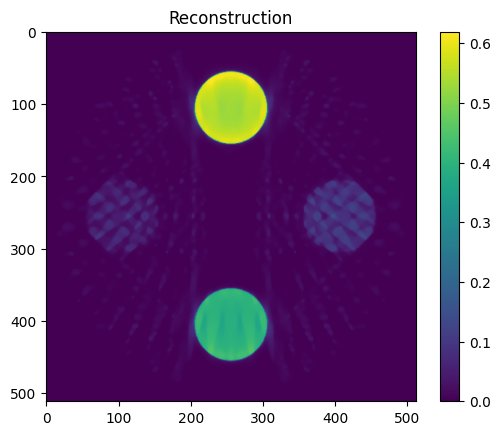
B01. FBP Reconstruction using LEAP¶

Reconstructing one CT scan using FBP/RWLS.

[17]:

leapct = tomographicModels()
leapct.about()

leapct.set_conebeam(ct_info['NViews'],
                    ct_info["shape"][0],
                    ct_info["shape"][1],
                    ct_info["psize"][0],
                    ct_info["psize"][1],
                    0.5*(ct_info["shape"][0]-1),
                    0.5*(ct_info["shape"][1]-1),
                    leapct.setAngleArray(ct_info['NViews'], 360.0),
                    ct_info["SOD"],
                    ct_info["SDD"])

leapct.set_default_volume()
# Reconstructing one CT scan using FBP/RWLS.
sino = -np.log(trans_list[-1]).astype(np.float32)
sino = np.ascontiguousarray(sino, dtype=np.float32) # shape is numAngles, numRows, numCols
recon = leapct.allocate_volume() # shape is numZ, numY, numX
recon[:] = 0.0

startTime = time.time()
#leapct.backproject(g,f)
leapct.FBP(sino,recon)
filters = filterSequence(1.0e0) # filter strength argument must be turned to your specific application
filters.append(TV(leapct, delta=0.02/20.0)) # the delta argument must be turned to your specific application
leapct.RWLS(sino,recon,20,filters,None,'SQS')
print('Reconstruction Elapsed Time: ' + str(time.time()-startTime))

RWLS iteration 1 of 20
        lambda = 0.541518
RWLS iteration 2 of 20
        lambda = 0.3469472
RWLS iteration 3 of 20
        lambda = 0.2867504
RWLS iteration 4 of 20
        lambda = 0.2613304
RWLS iteration 5 of 20
        lambda = 0.24231522
RWLS iteration 6 of 20
        lambda = 0.2291172
RWLS iteration 7 of 20
        lambda = 0.21515176
RWLS iteration 8 of 20
        lambda = 0.20481074
RWLS iteration 9 of 20
        lambda = 0.195452
RWLS iteration 10 of 20
        lambda = 0.18794225
RWLS iteration 11 of 20
        lambda = 0.18118744
RWLS iteration 12 of 20
        lambda = 0.17525595
RWLS iteration 13 of 20
        lambda = 0.16966107
RWLS iteration 14 of 20
        lambda = 0.16442218
RWLS iteration 15 of 20
        lambda = 0.15923582
RWLS iteration 16 of 20
        lambda = 0.15322512
RWLS iteration 17 of 20
        lambda = 0.14910358
RWLS iteration 18 of 20
        lambda = 0.14532383
RWLS iteration 19 of 20
        lambda = 0.14127181
RWLS iteration 20 of 20
        lambda = 0.1381174
Reconstruction Elapsed Time: 5.577737331390381

[18]:

recon.shape

[18]:

(50, 512, 512)

[19]:

plt.imshow(recon[25])
plt.colorbar()
plt.title('Reconstruction')

[19]:

Text(0.5, 1.0, 'Reconstruction')

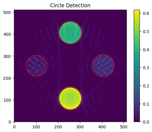
../_images/examples_T01_Calibration_LEAP_32_1.png

B02. Circle Detection (Optional)¶

The circle detection provides a coarse bounding box for object segmentation. One can manually set the bounding box for the object segmentation, if the sample is not cylindrical.

Below is an example to use detect_hough_circles to detect circles on the $25^{th}$ slice of the reconstruction.

[20]:

from xcal.phantom import detect_hough_circles

[21]:

help(detect_hough_circles)

Help on function detect_hough_circles in module xcal.phantom:

detect_hough_circles(phantom, radius_range=None, vmin=0, vmax=None, min_dist=100, HoughCircles_params1=300, HoughCircles_params2=1)
    Detects circles in an image using the Hough Circle Transform.

    Args:
        phantom (numpy.ndarray): The 2D image to detect circles in.
        radius_range (list of int, optional): The minimum and maximum radius of
            circles to detect. Defaults to a range based on the image size.
        vmin (int, optional): Minimum value for clipping the image before
            detection. Defaults to 0.
        vmax (int, optional): Maximum value for clipping the image before
            detection. If None, the 90th percentile of the image is used.
            Defaults to None.
        min_dist (int, optional): Minimum distance between the centers of the
            detected circles. If too small, multiple neighbor circles may be
            falsely detected in addition to a true one. If too large, some
            circles may be missed. Defaults to 100.
        HoughCircles_params1 (float, optional): Upper threshold for the internal edge detection.
        HoughCircles_params2 (float, optional): Threshold for center detection, which influences the detection sensitivity. Large param2 leads to fewer detected circles.

    Returns:
        numpy.ndarray: An array of detected circles, each represented by the
            center coordinates (x, y) and radius. Returns an empty array if no
            circles are detected.

[22]:

from matplotlib.patches import Circle
import math

plt.imshow(recon[25],origin='lower')
plt.colorbar()
# Get the current axes.
ax = plt.gca()
circles = detect_hough_circles(recon[25],
                               radius_range=(45, 55),
                               vmin=0.00, vmax=0.02,
                               min_dist=200,
                               HoughCircles_params2=10)

# Below is for display and sort the detected circles.
# x is horizontal axis, y is vertical axis.
circles_values = np.array([np.mean(recon[25][int(y-r):int(y+r),int(x-r):int(x+r)]) for x,y,r in circles])
# Sort `circles` based on the order in `circles_values`
circles = [cir for _, cir in sorted(zip(circles_values, circles))]
# Rearrange based on material ['V', 'Al', 'Ti', 'Mg']
circles = [circles[i] for i in [3,1,2,0]]

# Create and add circles to the plot.
for x, y, radius in circles:
    circle = Circle((x, y), radius, color='red', fill=False)
    ax.add_patch(circle)

# Optionally set the aspect of the plot to be equal.
# This makes sure that the circles are not skewed.
ax.set_aspect('equal')
plt.title('Circle Detection')
# Show the plot with the circles.
plt.show()

../_images/examples_T01_Calibration_LEAP_36_0.png

B03. Segment Object to get 3D Mask¶

segment_object is a function to segment one sample from background.

[23]:

from xcal.phantom import segment_object

[24]:

help(segment_object)

Help on function segment_object in module xcal.phantom:

segment_object(phantom, vmin, vmax, canny_sigma, roi_radius=None, bbox=None)
    Segments an object within a given region of interest (ROI) or bounding box in an image.

    This function creates a segmentation mask for an object in an image. The image values
    are clipped and normalized based on provided minimum and maximum values. Canny edge
    detection is then applied to the normalized image. The edges are filled to create a
    binary mask that segments the object.

    Args:
        phantom (np.array): The input image to segment.
        vmin (float): The minimum value for clipping the image.
        vmax (float): The maximum value for clipping the image.
        canny_sigma (float): The standard deviation for the Gaussian filter used in
                             Canny edge detection.
        roi_radius (int, optional): The radius of the circular region of interest. If not
                                    provided, it defaults to half the image size.
        bbox (tuple of int, optional): The bounding box within which to perform segmentation,
                                       specified as (r_min, c_min, r_max, c_max). If not
                                       provided, the entire image is used.

    Returns:
        np.array: A binary segmentation mask of the object.

[25]:

est_mask_list = []
bbox_half_size = int(np.mean([cir[2] for cir in circles])*1.1)
# Manually set the threshold based on above plot.
vmin_list = [0.02,0.01,0.2,0.01]
vmax_list = [0.7,0.02,0.4,0.02]
# Loop through each slice to get 3D mask.
for vi,cir in enumerate(circles):
    xcenter, ycenter, r = cir
    # Segment object with 3D mask
    # Set different vmin and vmax for different samples.
    # Set bbox to restrict a box region for object segmentation.
    est_mask = [segment_object(
        recon[i],
        vmin_list[vi],
        vmax_list[vi],
        10, # Canny sigma in canny edge detection. Larger value is more possible to connect to a line.
        roi_radius=None,
        bbox=(
            int(ycenter - bbox_half_size),
            int(xcenter - bbox_half_size),
            int(ycenter + bbox_half_size),
            int(xcenter + bbox_half_size)
        )) for i in range(len(recon))]
    est_mask_list.append(np.array(est_mask))

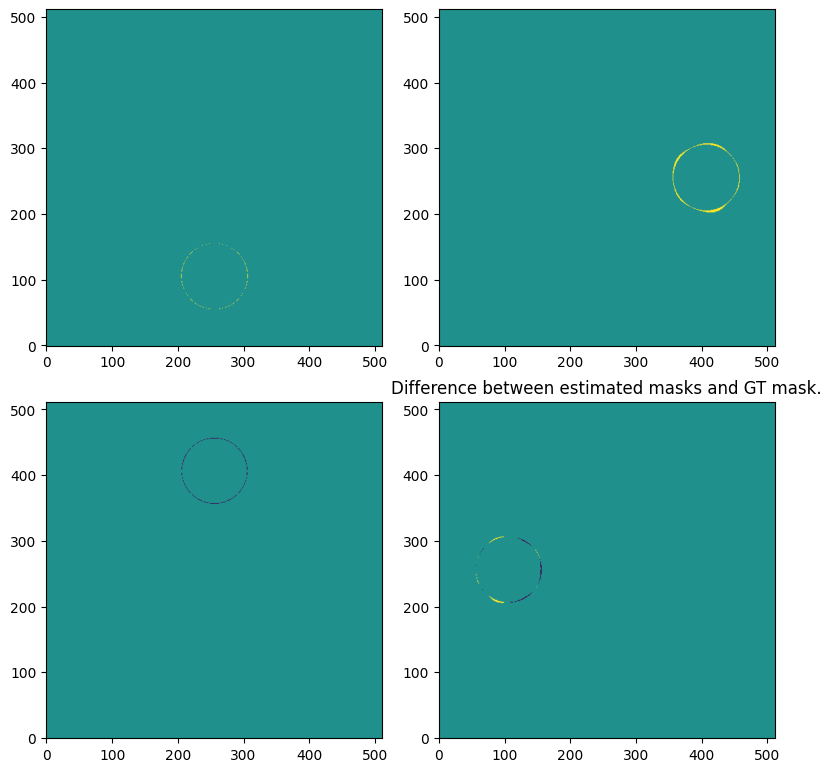
[26]:

fig, axs = plt.subplots(2, 2, figsize=(8, 8))

for j in range(len(est_mask_list)):
    ax = axs.flat[j]
    est_mask = est_mask_list[j]
    gtmask = mask_list[j]
    # Display the image or the difference image.
#     ax.imshow(est_mask[25],origin='lower')
    ax.imshow(est_mask[25].astype('float32')-gtmask[25].astype('float32'),vmin=-1,vmax=1,origin='lower')
# Adjust the layout
plt.tight_layout()
plt.title('Difference between estimated masks and GT mask.')
plt.show()

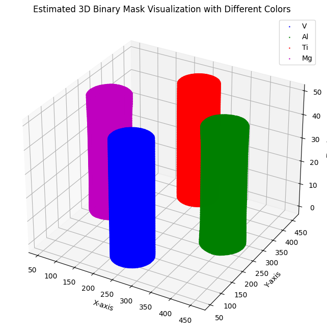
../_images/examples_T01_Calibration_LEAP_41_0.png

[27]:

# Define colors for each mask
colors = ['b', 'g', 'r', 'm']  # Blue, Green, Red, Magenta for each est_mask

# Plot the 3D masks using a scatter plot with different colors
fig = plt.figure(figsize=(8, 8))
ax = fig.add_subplot(111, projection='3d')

for i, est_mask in enumerate(est_mask_list):
    # Get the coordinates of the points where the mask is 1
    z, y, x = np.where(est_mask == 1)
    ax.scatter(x, y, z, color=colors[i], marker='o', s=1, alpha=0.7, label=sample_mats[i])

# Set labels and title
ax.set_xlabel("X-axis")
ax.set_ylabel("Y-axis")
ax.set_zlabel("Z-axis")
ax.set_title("Estimated 3D Binary Mask Visualization with Different Colors")
plt.legend()
plt.show()

../_images/examples_T01_Calibration_LEAP_42_0.png

B04. Calculate Forward Matrix with Estimated 3D Masks¶

[28]:

# Only use 8 different views for spectral calibration
NViews_For_MBSC = 8
calib_angles = leapct.setAngleArray(ct_info['NViews'], 360.0)[::ct_info["NViews"]//NViews_For_MBSC]
calib_angles = np.ascontiguousarray(calib_angles.astype(np.float32), dtype=np.float32)
projector2 =fw_projector(NViews_For_MBSC,
                        ct_info["shape"][0],
                        ct_info["shape"][1],
                        ct_info["psize"][0],
                        ct_info["psize"][1],
                        0.5*(ct_info["shape"][0]-1),
                        0.5*(ct_info["shape"][1]-1),
                        calib_angles,
                        ct_info["SOD"],
                        ct_info["SDD"])

[29]:

est_spec_F = calc_forward_matrix(est_mask_list, lac_vs_E_list, projector2)

Forward Projection Elapsed Time: 0.012677669525146484
Forward Projection Elapsed Time: 0.011296510696411133
Forward Projection Elapsed Time: 0.011538028717041016
Forward Projection Elapsed Time: 0.011275291442871094

B05. X-ray System Model Configuration¶

[30]:

from xcal.models import Reflection_Source, Filter, Scintillator
from xcal.defs import Material

[31]:

# Use Spekpy to generate a source spectra dictionary.
takeoff_angles = np.linspace(5,45,11)
src_spec_list = []
for case_i,simkV in enumerate(voltage_list):
    for ta in takeoff_angles:
        # Generate the X-ray spectrum model with Spekpy for each voltage.
        s = sp.Spek(kvp=simkV, th=ta, dk=1, z=ct_info['SDD'], mas=mas_list[case_i], char=True)
        k, phi_k = s.get_spectrum(edges=False)  # Retrieve energy bins and fluence spectrum [Photons cm^-2 keV^-1]

        # Adjust the fluence for the detector pixel area.
        phi_k = phi_k * ((ct_info['psize'][0] / 10) * (ct_info['psize'][1] / 10))  # Convert pixel size from mm² to cm²

        # Initialize a zero-filled spectrum array with length max_simkV.
        src_spec = np.zeros(max_simkV-1)
        src_spec[:simkV-1] = phi_k  # Assign spectrum values starting from 1.5 keV

        # Add the processed spectrum for this voltage to the list.
        src_spec_list.append(src_spec)

src_spec_list = np.array(src_spec_list)
src_spec_list = src_spec_list.reshape((len(voltage_list),len(takeoff_angles),-1))

[32]:

# Configure the Reflection Source Model
# Reflection_Source is a PyTorch module that supports gradient descent.
# Reflection_Source initializes with specified source voltage and takeoff angle.
# The set_src_spec_list method assigns a dictionary for each source configuration.
# Reflection_Source.forward() provides interpolated dictionary components for each source.

# Source voltage is set to be fixed by setting minbound and maxbound to None.
# Takeoff angle is estimated in range [5,45] with inital value 25 degree.
sources = [Reflection_Source(voltage=(voltage, None, None), takeoff_angle=(25, 5, 45), single_takeoff_angle=True)
           for voltage in voltage_list]
# Assigning the dictionaries for each source.
for src_i, source in enumerate(sources):
    source.set_src_spec_list(energies, src_spec_list, voltage_list, takeoff_angles)

[33]:

# Both the filter and scintillator contain discrete and continuous parameters.
# All continuous parameters are defined using a tuple format with an initial value, minimum bound, and maximum bound.
# Any other format is recognized as a discrete parameter.
# Concatenating all component instances (sources, filters, scintillator) into a list, called spectral configuration like [source, filter_1, scintillator_1],
# allows the Estimator defined in B07 to recognize all parameters, whether discrete or continuous for a scan.
# The spec_models collects all spectral configuration. Each spectral configuration corresponding to a scan.
# The Estimator will then automatically determine all possible combinations for the discrete parameters and optimize the continous parameters.


# Configure Filter Model
# Knowns: Use one filter for both scans.
# Possible filter materials: Al and Cu.
psb_fltr_mat = [Material(formula='Al', density=2.702),
                Material(formula='Cu', density=8.92)]
filter_1 = Filter(psb_fltr_mat, thickness=(5, 0, 10))

# Configure Scintillator Model
# Knowns: Use one scintillator for both scans.
# Possible scintillator materials
scint_params_list = [
    {'formula': 'CsI', 'density': 4.51},
    {'formula': 'Gd3Al2Ga3O12', 'density': 6.63},
    {'formula': 'Lu3Al5O12', 'density': 6.73},
    {'formula': 'CdWO4', 'density': 7.9},
    {'formula': 'Y3Al5O12', 'density': 4.56},
    {'formula': 'Bi4Ge3O12', 'density': 7.13},
    {'formula': 'Gd2O2S', 'density': 7.32}
]
psb_scint_mat = [Material(formula=scint_p['formula'], density=scint_p['density']) for scint_p in scint_params_list]
scintillator_1 = Scintillator(materials=psb_scint_mat, thickness=(0.25, 0.01, 0.5))

# For each scan using a different source voltage, we define a different total spectral model.
# Each spectral model is a list containing source, filters, and scintillator models.
# Allow filter_1, ..., filter_n.
spec_models = [[source, filter_1, scintillator_1] for source in sources]

B06. Spectral Calibration with Simulated Multi-Energy Data¶

[34]:

# Build Training Set
# Use first 8 views and center 2 slices.
train_rads = [trans[::ct_info["NViews"]//NViews_For_MBSC,10:-10:10] for trans in trans_list]

# Assume a same forward matrix for different scans at different voltages.
forward_matrices = [est_spec_F[:,10:-10:10] for i in range(len(voltage_list))]

print("Training Measurement Shape: \n", train_rads[0].shape,train_rads[1].shape,train_rads[2].shape)
print("Training Forward Matrix Shape: \n",forward_matrices[0].shape,forward_matrices[1].shape,forward_matrices[2].shape)

Training Measurement Shape:
 (8, 3, 512) (8, 3, 512) (8, 3, 512)
Training Forward Matrix Shape:
 (8, 3, 512, 179) (8, 3, 512, 179) (8, 3, 512, 179)

[35]:

from xcal.estimate import Estimate

learning_rate = 0.01 # 0.01 for NNAT_LBFGS and 0.001 for Adam
max_iterations = 5000 # 5000 ~ 10000 would be enough
stop_threshold = 1e-6
optimizer_type = 'NNAT_LBFGS' # Can also use Adam.

Estimator = Estimate(energies)
# For each scan, add data and calculated forward matrix to Estimator.
for nrad, forward_matrix, concatenate_models in zip(train_rads, forward_matrices, spec_models):
    Estimator.add_data(nrad, forward_matrix, concatenate_models, weight=None)

# Fit data
Estimator.fit(learning_rate=learning_rate,
              max_iterations=max_iterations,
              stop_threshold=stop_threshold,
              optimizer_type=optimizer_type,
              loss_type='transmission',
              logpath=None,
              num_processes=1) # Parallel computing for multiple cpus.

Number of cases for different discrete parameters: 14

2025-05-07 01:28:03,034  - Start Estimation.
2025-05-07 01:28:03,295  - Initial cost: 1.587707e-03
2025-05-07 01:28:05,063  - Iteration: 5
2025-05-07 01:28:05,335  - Cost: 0.0006723980768583715
2025-05-07 01:28:05,336  - Filter_2_material: Material(formula='Al', density=2.702)
2025-05-07 01:28:05,336  - Filter_2_thickness: 4.213513374328613
2025-05-07 01:28:05,336  - Reflection_Source_1_voltage: 40.0
2025-05-07 01:28:05,336  - Reflection_Source_2_voltage: 80.0
2025-05-07 01:28:05,336  - Reflection_Source_3_voltage: 180.0
2025-05-07 01:28:05,336  - Reflection_Source_takeoff_angle: 25.23719596862793
2025-05-07 01:28:05,336  - Scintillator_2_material: Material(formula='CsI', density=4.51)
2025-05-07 01:28:05,336  - Scintillator_2_thickness: 0.25396865606307983
2025-05-07 01:28:05,336  -
2025-05-07 01:28:06,458  - Iteration: 10
2025-05-07 01:28:06,739  - Cost: 0.0005372301675379276
2025-05-07 01:28:06,739  - Filter_2_material: Material(formula='Al', density=2.702)
2025-05-07 01:28:06,739  - Filter_2_thickness: 3.917762279510498
2025-05-07 01:28:06,739  - Reflection_Source_1_voltage: 40.0
2025-05-07 01:28:06,739  - Reflection_Source_2_voltage: 80.0
2025-05-07 01:28:06,739  - Reflection_Source_3_voltage: 180.0
2025-05-07 01:28:06,739  - Reflection_Source_takeoff_angle: 24.901470184326172
2025-05-07 01:28:06,739  - Scintillator_2_material: Material(formula='CsI', density=4.51)
2025-05-07 01:28:06,740  - Scintillator_2_thickness: 0.26431193947792053
2025-05-07 01:28:06,740  -
2025-05-07 01:28:07,843  - Iteration: 15
2025-05-07 01:28:08,107  - Cost: 0.0004892278229817748
2025-05-07 01:28:08,107  - Filter_2_material: Material(formula='Al', density=2.702)
2025-05-07 01:28:08,107  - Filter_2_thickness: 3.723284959793091
2025-05-07 01:28:08,107  - Reflection_Source_1_voltage: 40.0
2025-05-07 01:28:08,107  - Reflection_Source_2_voltage: 80.0
2025-05-07 01:28:08,107  - Reflection_Source_3_voltage: 180.0
2025-05-07 01:28:08,107  - Reflection_Source_takeoff_angle: 24.221975326538086
2025-05-07 01:28:08,108  - Scintillator_2_material: Material(formula='CsI', density=4.51)
2025-05-07 01:28:08,108  - Scintillator_2_thickness: 0.2807618975639343
2025-05-07 01:28:08,108  -
2025-05-07 01:28:09,133  - Iteration: 20
2025-05-07 01:28:09,441  - Cost: 0.0004244772717356682
2025-05-07 01:28:09,441  - Filter_2_material: Material(formula='Al', density=2.702)
2025-05-07 01:28:09,441  - Filter_2_thickness: 3.4932219982147217
2025-05-07 01:28:09,441  - Reflection_Source_1_voltage: 40.0
2025-05-07 01:28:09,441  - Reflection_Source_2_voltage: 80.0
2025-05-07 01:28:09,441  - Reflection_Source_3_voltage: 180.0
2025-05-07 01:28:09,442  - Reflection_Source_takeoff_angle: 22.232118606567383
2025-05-07 01:28:09,442  - Scintillator_2_material: Material(formula='CsI', density=4.51)
2025-05-07 01:28:09,442  - Scintillator_2_thickness: 0.3217521011829376
2025-05-07 01:28:09,442  -
2025-05-07 01:28:10,528  - Iteration: 25
2025-05-07 01:28:10,788  - Cost: 0.00037808914203196764
2025-05-07 01:28:10,788  - Filter_2_material: Material(formula='Al', density=2.702)
2025-05-07 01:28:10,788  - Filter_2_thickness: 3.3206706047058105
2025-05-07 01:28:10,789  - Reflection_Source_1_voltage: 40.0
2025-05-07 01:28:10,789  - Reflection_Source_2_voltage: 80.0
2025-05-07 01:28:10,789  - Reflection_Source_3_voltage: 180.0
2025-05-07 01:28:10,789  - Reflection_Source_takeoff_angle: 19.43391227722168
2025-05-07 01:28:10,789  - Scintillator_2_material: Material(formula='CsI', density=4.51)
2025-05-07 01:28:10,789  - Scintillator_2_thickness: 0.3617841303348541
2025-05-07 01:28:10,789  -
2025-05-07 01:28:11,846  - Iteration: 30
2025-05-07 01:28:11,934  - Cost: 0.00037053183768875897
2025-05-07 01:28:11,934  - Filter_2_material: Material(formula='Al', density=2.702)
2025-05-07 01:28:11,934  - Filter_2_thickness: 3.2547454833984375
2025-05-07 01:28:11,934  - Reflection_Source_1_voltage: 40.0
2025-05-07 01:28:11,934  - Reflection_Source_2_voltage: 80.0
2025-05-07 01:28:11,935  - Reflection_Source_3_voltage: 180.0
2025-05-07 01:28:11,935  - Reflection_Source_takeoff_angle: 18.24373435974121
2025-05-07 01:28:11,935  - Scintillator_2_material: Material(formula='CsI', density=4.51)
2025-05-07 01:28:11,935  - Scintillator_2_thickness: 0.37452903389930725
2025-05-07 01:28:11,935  -
2025-05-07 01:28:13,000  - Iteration: 35
2025-05-07 01:28:13,259  - Cost: 0.0003688415454234928
2025-05-07 01:28:13,260  - Filter_2_material: Material(formula='Al', density=2.702)
2025-05-07 01:28:13,260  - Filter_2_thickness: 3.212918281555176
2025-05-07 01:28:13,260  - Reflection_Source_1_voltage: 40.0
2025-05-07 01:28:13,260  - Reflection_Source_2_voltage: 80.0
2025-05-07 01:28:13,260  - Reflection_Source_3_voltage: 180.0
2025-05-07 01:28:13,260  - Reflection_Source_takeoff_angle: 17.559783935546875
2025-05-07 01:28:13,260  - Scintillator_2_material: Material(formula='CsI', density=4.51)
2025-05-07 01:28:13,260  - Scintillator_2_thickness: 0.38003554940223694
2025-05-07 01:28:13,260  -
2025-05-07 01:28:14,334  - Iteration: 40
2025-05-07 01:28:14,596  - Cost: 0.00036846011062152684
2025-05-07 01:28:14,597  - Filter_2_material: Material(formula='Al', density=2.702)
2025-05-07 01:28:14,597  - Filter_2_thickness: 3.189002513885498
2025-05-07 01:28:14,597  - Reflection_Source_1_voltage: 40.0
2025-05-07 01:28:14,597  - Reflection_Source_2_voltage: 80.0
2025-05-07 01:28:14,597  - Reflection_Source_3_voltage: 180.0
2025-05-07 01:28:14,597  - Reflection_Source_takeoff_angle: 17.103303909301758
2025-05-07 01:28:14,597  - Scintillator_2_material: Material(formula='CsI', density=4.51)
2025-05-07 01:28:14,597  - Scintillator_2_thickness: 0.3803960978984833
2025-05-07 01:28:14,597  -
2025-05-07 01:28:15,543  - Iteration: 45
2025-05-07 01:28:15,967  - Cost: 0.00036830356111750007
2025-05-07 01:28:15,967  - Filter_2_material: Material(formula='Al', density=2.702)
2025-05-07 01:28:15,967  - Filter_2_thickness: 3.1706764698028564
2025-05-07 01:28:15,967  - Reflection_Source_1_voltage: 40.0
2025-05-07 01:28:15,967  - Reflection_Source_2_voltage: 80.0
2025-05-07 01:28:15,967  - Reflection_Source_3_voltage: 180.0
2025-05-07 01:28:15,968  - Reflection_Source_takeoff_angle: 16.706764221191406
2025-05-07 01:28:15,968  - Scintillator_2_material: Material(formula='CsI', density=4.51)
2025-05-07 01:28:15,968  - Scintillator_2_thickness: 0.3783363997936249
2025-05-07 01:28:15,968  -
2025-05-07 01:28:16,964  - Iteration: 50
2025-05-07 01:28:17,220  - Cost: 0.000368042616173625
2025-05-07 01:28:17,221  - Filter_2_material: Material(formula='Al', density=2.702)
2025-05-07 01:28:17,221  - Filter_2_thickness: 3.1412482261657715
2025-05-07 01:28:17,221  - Reflection_Source_1_voltage: 40.0
2025-05-07 01:28:17,221  - Reflection_Source_2_voltage: 80.0
2025-05-07 01:28:17,221  - Reflection_Source_3_voltage: 180.0
2025-05-07 01:28:17,221  - Reflection_Source_takeoff_angle: 15.944174766540527
2025-05-07 01:28:17,221  - Scintillator_2_material: Material(formula='CsI', density=4.51)
2025-05-07 01:28:17,221  - Scintillator_2_thickness: 0.36924588680267334
2025-05-07 01:28:17,221  -
2025-05-07 01:28:18,165  - Iteration: 55
2025-05-07 01:28:18,422  - Cost: 0.00036780975642614067
2025-05-07 01:28:18,423  - Filter_2_material: Material(formula='Al', density=2.702)
2025-05-07 01:28:18,423  - Filter_2_thickness: 3.1230220794677734
2025-05-07 01:28:18,423  - Reflection_Source_1_voltage: 40.0
2025-05-07 01:28:18,423  - Reflection_Source_2_voltage: 80.0
2025-05-07 01:28:18,423  - Reflection_Source_3_voltage: 180.0
2025-05-07 01:28:18,423  - Reflection_Source_takeoff_angle: 15.295877456665039
2025-05-07 01:28:18,423  - Scintillator_2_material: Material(formula='CsI', density=4.51)
2025-05-07 01:28:18,424  - Scintillator_2_thickness: 0.3571985065937042
2025-05-07 01:28:18,424  -
2025-05-07 01:28:19,409  - Iteration: 60
2025-05-07 01:28:19,775  - Cost: 0.00036774860927835107
2025-05-07 01:28:19,775  - Filter_2_material: Material(formula='Al', density=2.702)
2025-05-07 01:28:19,776  - Filter_2_thickness: 3.1128337383270264
2025-05-07 01:28:19,776  - Reflection_Source_1_voltage: 40.0
2025-05-07 01:28:19,776  - Reflection_Source_2_voltage: 80.0
2025-05-07 01:28:19,776  - Reflection_Source_3_voltage: 180.0
2025-05-07 01:28:19,776  - Reflection_Source_takeoff_angle: 14.917986869812012
2025-05-07 01:28:19,776  - Scintillator_2_material: Material(formula='CsI', density=4.51)
2025-05-07 01:28:19,776  - Scintillator_2_thickness: 0.35052624344825745
2025-05-07 01:28:19,776  -
2025-05-07 01:28:20,831  - Iteration: 65
2025-05-07 01:28:21,097  - Cost: 0.0003677362692542374
2025-05-07 01:28:21,097  - Filter_2_material: Material(formula='Al', density=2.702)
2025-05-07 01:28:21,097  - Filter_2_thickness: 3.1076555252075195
2025-05-07 01:28:21,097  - Reflection_Source_1_voltage: 40.0
2025-05-07 01:28:21,097  - Reflection_Source_2_voltage: 80.0
2025-05-07 01:28:21,097  - Reflection_Source_3_voltage: 180.0
2025-05-07 01:28:21,097  - Reflection_Source_takeoff_angle: 14.74304485321045
2025-05-07 01:28:21,097  - Scintillator_2_material: Material(formula='CsI', density=4.51)
2025-05-07 01:28:21,097  - Scintillator_2_thickness: 0.3474627435207367
2025-05-07 01:28:21,097  -
2025-05-07 01:28:26,326  - Stopping at epoch 69 because updates are too small.
2025-05-07 01:28:26,327  - Cost: 0.00036773463943973184
2025-05-07 01:28:26,327  - Filter_2_material: Material(formula='Al', density=2.702)
2025-05-07 01:28:26,327  - Filter_2_thickness: 3.106395959854126
2025-05-07 01:28:26,327  - Reflection_Source_1_voltage: 40.0
2025-05-07 01:28:26,327  - Reflection_Source_2_voltage: 80.0
2025-05-07 01:28:26,327  - Reflection_Source_3_voltage: 180.0
2025-05-07 01:28:26,327  - Reflection_Source_takeoff_angle: 14.694992065429688
2025-05-07 01:28:26,327  - Scintillator_2_material: Material(formula='CsI', density=4.51)
2025-05-07 01:28:26,327  - Scintillator_2_thickness: 0.3465994596481323
2025-05-07 01:28:26,327  -
2025-05-07 01:28:26,344  - Start Estimation.
2025-05-07 01:28:26,455  - Initial cost: 2.492245e-03
2025-05-07 01:28:27,683  - Iteration: 5
2025-05-07 01:28:27,987  - Cost: 0.0022279920522123575
2025-05-07 01:28:27,987  - Filter_2_material: Material(formula='Al', density=2.702)
2025-05-07 01:28:27,988  - Filter_2_thickness: 4.5608134269714355
2025-05-07 01:28:27,988  - Reflection_Source_1_voltage: 40.0
2025-05-07 01:28:27,988  - Reflection_Source_2_voltage: 80.0
2025-05-07 01:28:27,988  - Reflection_Source_3_voltage: 180.0
2025-05-07 01:28:27,988  - Reflection_Source_takeoff_angle: 24.26715660095215
2025-05-07 01:28:27,988  - Scintillator_2_material: Material(formula='Gd3Al2Ga3O12', density=6.63)
2025-05-07 01:28:27,988  - Scintillator_2_thickness: 0.24550770223140717
2025-05-07 01:28:27,988  -
2025-05-07 01:28:29,093  - Iteration: 10
2025-05-07 01:28:29,369  - Cost: 0.0020399701315909624
2025-05-07 01:28:29,369  - Filter_2_material: Material(formula='Al', density=2.702)
2025-05-07 01:28:29,369  - Filter_2_thickness: 4.043423652648926
2025-05-07 01:28:29,369  - Reflection_Source_1_voltage: 40.0
2025-05-07 01:28:29,369  - Reflection_Source_2_voltage: 80.0
2025-05-07 01:28:29,370  - Reflection_Source_3_voltage: 180.0
2025-05-07 01:28:29,370  - Reflection_Source_takeoff_angle: 20.537090301513672
2025-05-07 01:28:29,370  - Scintillator_2_material: Material(formula='Gd3Al2Ga3O12', density=6.63)
2025-05-07 01:28:29,370  - Scintillator_2_thickness: 0.24091015756130219
2025-05-07 01:28:29,370  -
2025-05-07 01:28:36,547  - Stopping at epoch 12 because updates are too small.
2025-05-07 01:28:36,547  - Cost: 0.0018955550622195005
2025-05-07 01:28:36,547  - Filter_2_material: Material(formula='Al', density=2.702)
2025-05-07 01:28:36,547  - Filter_2_thickness: 3.614506959915161
2025-05-07 01:28:36,547  - Reflection_Source_1_voltage: 40.0
2025-05-07 01:28:36,547  - Reflection_Source_2_voltage: 80.0
2025-05-07 01:28:36,547  - Reflection_Source_3_voltage: 180.0
2025-05-07 01:28:36,547  - Reflection_Source_takeoff_angle: 16.471574783325195
2025-05-07 01:28:36,548  - Scintillator_2_material: Material(formula='Gd3Al2Ga3O12', density=6.63)
2025-05-07 01:28:36,548  - Scintillator_2_thickness: 0.23732063174247742
2025-05-07 01:28:36,548  -
2025-05-07 01:28:36,556  - Start Estimation.
2025-05-07 01:28:36,626  - Initial cost: 3.077974e-03
2025-05-07 01:28:37,763  - Iteration: 5
2025-05-07 01:28:38,021  - Cost: 0.0028075443115085363
2025-05-07 01:28:38,021  - Filter_2_material: Material(formula='Al', density=2.702)
2025-05-07 01:28:38,021  - Filter_2_thickness: 4.450414180755615
2025-05-07 01:28:38,021  - Reflection_Source_1_voltage: 40.0
2025-05-07 01:28:38,021  - Reflection_Source_2_voltage: 80.0
2025-05-07 01:28:38,022  - Reflection_Source_3_voltage: 180.0
2025-05-07 01:28:38,022  - Reflection_Source_takeoff_angle: 23.74559783935547
2025-05-07 01:28:38,022  - Scintillator_2_material: Material(formula='Lu3Al5O12', density=6.73)
2025-05-07 01:28:38,022  - Scintillator_2_thickness: 0.2595919072628021
2025-05-07 01:28:38,022  -
2025-05-07 01:28:39,071  - Iteration: 10
2025-05-07 01:28:39,313  - Cost: 0.002328362548723817
2025-05-07 01:28:39,313  - Filter_2_material: Material(formula='Al', density=2.702)
2025-05-07 01:28:39,313  - Filter_2_thickness: 3.1984691619873047
2025-05-07 01:28:39,313  - Reflection_Source_1_voltage: 40.0
2025-05-07 01:28:39,313  - Reflection_Source_2_voltage: 80.0
2025-05-07 01:28:39,313  - Reflection_Source_3_voltage: 180.0
2025-05-07 01:28:39,313  - Reflection_Source_takeoff_angle: 16.630538940429688
2025-05-07 01:28:39,313  - Scintillator_2_material: Material(formula='Lu3Al5O12', density=6.73)
2025-05-07 01:28:39,314  - Scintillator_2_thickness: 0.31992319226264954
2025-05-07 01:28:39,314  -
2025-05-07 01:28:44,460  - Stopping at epoch 13 because updates are too small.
2025-05-07 01:28:44,460  - Cost: 0.0020117536187171936
2025-05-07 01:28:44,460  - Filter_2_material: Material(formula='Al', density=2.702)
2025-05-07 01:28:44,460  - Filter_2_thickness: 2.4119725227355957
2025-05-07 01:28:44,460  - Reflection_Source_1_voltage: 40.0
2025-05-07 01:28:44,460  - Reflection_Source_2_voltage: 80.0
2025-05-07 01:28:44,461  - Reflection_Source_3_voltage: 180.0
2025-05-07 01:28:44,461  - Reflection_Source_takeoff_angle: 10.766779899597168
2025-05-07 01:28:44,461  - Scintillator_2_material: Material(formula='Lu3Al5O12', density=6.73)
2025-05-07 01:28:44,461  - Scintillator_2_thickness: 0.36598074436187744
2025-05-07 01:28:44,461  -
2025-05-07 01:28:44,468  - Start Estimation.
2025-05-07 01:28:44,584  - Initial cost: 3.022571e-03
2025-05-07 01:28:45,723  - Iteration: 5
2025-05-07 01:28:45,972  - Cost: 0.0013409802922978997
2025-05-07 01:28:45,973  - Filter_2_material: Material(formula='Al', density=2.702)
2025-05-07 01:28:45,973  - Filter_2_thickness: 3.805534601211548
2025-05-07 01:28:45,973  - Reflection_Source_1_voltage: 40.0
2025-05-07 01:28:45,973  - Reflection_Source_2_voltage: 80.0
2025-05-07 01:28:45,973  - Reflection_Source_3_voltage: 180.0
2025-05-07 01:28:45,973  - Reflection_Source_takeoff_angle: 24.96942710876465
2025-05-07 01:28:45,973  - Scintillator_2_material: Material(formula='CdWO4', density=7.9)
2025-05-07 01:28:45,973  - Scintillator_2_thickness: 0.2639610469341278
2025-05-07 01:28:45,973  -
2025-05-07 01:28:47,032  - Iteration: 10
2025-05-07 01:28:47,275  - Cost: 0.0009760453831404448
2025-05-07 01:28:47,276  - Filter_2_material: Material(formula='Al', density=2.702)
2025-05-07 01:28:47,276  - Filter_2_thickness: 3.228907823562622
2025-05-07 01:28:47,276  - Reflection_Source_1_voltage: 40.0
2025-05-07 01:28:47,276  - Reflection_Source_2_voltage: 80.0
2025-05-07 01:28:47,276  - Reflection_Source_3_voltage: 180.0
2025-05-07 01:28:47,276  - Reflection_Source_takeoff_angle: 23.93007469177246
2025-05-07 01:28:47,276  - Scintillator_2_material: Material(formula='CdWO4', density=7.9)
2025-05-07 01:28:47,276  - Scintillator_2_thickness: 0.29830750823020935
2025-05-07 01:28:47,276  -
2025-05-07 01:28:48,355  - Iteration: 15
2025-05-07 01:28:48,624  - Cost: 0.0007440934423357248
2025-05-07 01:28:48,624  - Filter_2_material: Material(formula='Al', density=2.702)
2025-05-07 01:28:48,624  - Filter_2_thickness: 2.812162399291992
2025-05-07 01:28:48,624  - Reflection_Source_1_voltage: 40.0
2025-05-07 01:28:48,624  - Reflection_Source_2_voltage: 80.0
2025-05-07 01:28:48,625  - Reflection_Source_3_voltage: 180.0
2025-05-07 01:28:48,625  - Reflection_Source_takeoff_angle: 21.70795249938965
2025-05-07 01:28:48,625  - Scintillator_2_material: Material(formula='CdWO4', density=7.9)
2025-05-07 01:28:48,625  - Scintillator_2_thickness: 0.35040944814682007
2025-05-07 01:28:48,625  -
2025-05-07 01:28:49,706  - Iteration: 20
2025-05-07 01:28:49,955  - Cost: 0.0004922390799038112
2025-05-07 01:28:49,956  - Filter_2_material: Material(formula='Al', density=2.702)
2025-05-07 01:28:49,956  - Filter_2_thickness: 2.4898428916931152
2025-05-07 01:28:49,956  - Reflection_Source_1_voltage: 40.0
2025-05-07 01:28:49,956  - Reflection_Source_2_voltage: 80.0
2025-05-07 01:28:49,956  - Reflection_Source_3_voltage: 180.0
2025-05-07 01:28:49,956  - Reflection_Source_takeoff_angle: 16.514972686767578
2025-05-07 01:28:49,956  - Scintillator_2_material: Material(formula='CdWO4', density=7.9)
2025-05-07 01:28:49,956  - Scintillator_2_thickness: 0.4168078303337097
2025-05-07 01:28:49,956  -
2025-05-07 01:28:50,954  - Iteration: 25
2025-05-07 01:28:51,034  - Cost: 0.0004464127996470779
2025-05-07 01:28:51,035  - Filter_2_material: Material(formula='Al', density=2.702)
2025-05-07 01:28:51,035  - Filter_2_thickness: 2.3622331619262695
2025-05-07 01:28:51,035  - Reflection_Source_1_voltage: 40.0
2025-05-07 01:28:51,035  - Reflection_Source_2_voltage: 80.0
2025-05-07 01:28:51,035  - Reflection_Source_3_voltage: 180.0
2025-05-07 01:28:51,035  - Reflection_Source_takeoff_angle: 14.109383583068848
2025-05-07 01:28:51,035  - Scintillator_2_material: Material(formula='CdWO4', density=7.9)
2025-05-07 01:28:51,035  - Scintillator_2_thickness: 0.4380587935447693
2025-05-07 01:28:51,035  -
2025-05-07 01:28:52,155  - Iteration: 30
2025-05-07 01:28:52,435  - Cost: 0.00043726476724259555
2025-05-07 01:28:52,436  - Filter_2_material: Material(formula='Al', density=2.702)
2025-05-07 01:28:52,436  - Filter_2_thickness: 2.3069417476654053
2025-05-07 01:28:52,436  - Reflection_Source_1_voltage: 40.0
2025-05-07 01:28:52,436  - Reflection_Source_2_voltage: 80.0
2025-05-07 01:28:52,436  - Reflection_Source_3_voltage: 180.0
2025-05-07 01:28:52,436  - Reflection_Source_takeoff_angle: 13.096059799194336
2025-05-07 01:28:52,436  - Scintillator_2_material: Material(formula='CdWO4', density=7.9)
2025-05-07 01:28:52,436  - Scintillator_2_thickness: 0.448375403881073
2025-05-07 01:28:52,436  -
2025-05-07 01:28:53,529  - Iteration: 35
2025-05-07 01:28:53,780  - Cost: 0.00043515473953448236
2025-05-07 01:28:53,781  - Filter_2_material: Material(formula='Al', density=2.702)
2025-05-07 01:28:53,781  - Filter_2_thickness: 2.2871174812316895
2025-05-07 01:28:53,781  - Reflection_Source_1_voltage: 40.0
2025-05-07 01:28:53,781  - Reflection_Source_2_voltage: 80.0
2025-05-07 01:28:53,781  - Reflection_Source_3_voltage: 180.0
2025-05-07 01:28:53,781  - Reflection_Source_takeoff_angle: 12.802369117736816
2025-05-07 01:28:53,781  - Scintillator_2_material: Material(formula='CdWO4', density=7.9)
2025-05-07 01:28:53,781  - Scintillator_2_thickness: 0.4561339318752289
2025-05-07 01:28:53,781  -
2025-05-07 01:28:54,669  - Iteration: 40
2025-05-07 01:28:54,943  - Cost: 0.00043402143637649715
2025-05-07 01:28:54,943  - Filter_2_material: Material(formula='Al', density=2.702)
2025-05-07 01:28:54,944  - Filter_2_thickness: 2.2812235355377197
2025-05-07 01:28:54,944  - Reflection_Source_1_voltage: 40.0
2025-05-07 01:28:54,944  - Reflection_Source_2_voltage: 80.0
2025-05-07 01:28:54,944  - Reflection_Source_3_voltage: 180.0
2025-05-07 01:28:54,944  - Reflection_Source_takeoff_angle: 12.808342933654785
2025-05-07 01:28:54,944  - Scintillator_2_material: Material(formula='CdWO4', density=7.9)
2025-05-07 01:28:54,944  - Scintillator_2_thickness: 0.46502411365509033
2025-05-07 01:28:54,944  -
2025-05-07 01:28:56,019  - Iteration: 45
2025-05-07 01:28:56,261  - Cost: 0.00043026055209338665
2025-05-07 01:28:56,261  - Filter_2_material: Material(formula='Al', density=2.702)
2025-05-07 01:28:56,261  - Filter_2_thickness: 2.299126625061035
2025-05-07 01:28:56,261  - Reflection_Source_1_voltage: 40.0
2025-05-07 01:28:56,261  - Reflection_Source_2_voltage: 80.0
2025-05-07 01:28:56,261  - Reflection_Source_3_voltage: 180.0
2025-05-07 01:28:56,261  - Reflection_Source_takeoff_angle: 13.916543960571289
2025-05-07 01:28:56,261  - Scintillator_2_material: Material(formula='CdWO4', density=7.9)
2025-05-07 01:28:56,262  - Scintillator_2_thickness: 0.49995315074920654
2025-05-07 01:28:56,262  -
2025-05-07 01:29:01,141  - Stopping at epoch 46 because updates are too small.
2025-05-07 01:29:01,141  - Cost: 0.00043026095954701304
2025-05-07 01:29:01,141  - Filter_2_material: Material(formula='Al', density=2.702)
2025-05-07 01:29:01,141  - Filter_2_thickness: 2.299126625061035
2025-05-07 01:29:01,141  - Reflection_Source_1_voltage: 40.0
2025-05-07 01:29:01,141  - Reflection_Source_2_voltage: 80.0
2025-05-07 01:29:01,141  - Reflection_Source_3_voltage: 180.0
2025-05-07 01:29:01,142  - Reflection_Source_takeoff_angle: 13.91654109954834
2025-05-07 01:29:01,142  - Scintillator_2_material: Material(formula='CdWO4', density=7.9)
2025-05-07 01:29:01,142  - Scintillator_2_thickness: 0.49995318055152893
2025-05-07 01:29:01,142  -
2025-05-07 01:29:01,150  - Start Estimation.
2025-05-07 01:29:01,219  - Initial cost: 5.902383e-03
2025-05-07 01:29:02,280  - Iteration: 5
2025-05-07 01:29:02,515  - Cost: 0.0054838890209794044
2025-05-07 01:29:02,515  - Filter_2_material: Material(formula='Al', density=2.702)
2025-05-07 01:29:02,515  - Filter_2_thickness: 5.216713905334473
2025-05-07 01:29:02,515  - Reflection_Source_1_voltage: 40.0
2025-05-07 01:29:02,515  - Reflection_Source_2_voltage: 80.0
2025-05-07 01:29:02,515  - Reflection_Source_3_voltage: 180.0
2025-05-07 01:29:02,515  - Reflection_Source_takeoff_angle: 22.25094223022461
2025-05-07 01:29:02,516  - Scintillator_2_material: Material(formula='Y3Al5O12', density=4.56)
2025-05-07 01:29:02,516  - Scintillator_2_thickness: 0.27568092942237854
2025-05-07 01:29:02,516  -
2025-05-07 01:29:03,510  - Iteration: 10
2025-05-07 01:29:03,782  - Cost: 0.004397060256451368
2025-05-07 01:29:03,782  - Filter_2_material: Material(formula='Al', density=2.702)
2025-05-07 01:29:03,783  - Filter_2_thickness: 4.727838516235352
2025-05-07 01:29:03,783  - Reflection_Source_1_voltage: 40.0
2025-05-07 01:29:03,783  - Reflection_Source_2_voltage: 80.0
2025-05-07 01:29:03,783  - Reflection_Source_3_voltage: 180.0
2025-05-07 01:29:03,783  - Reflection_Source_takeoff_angle: 8.110776901245117
2025-05-07 01:29:03,783  - Scintillator_2_material: Material(formula='Y3Al5O12', density=4.56)
2025-05-07 01:29:03,783  - Scintillator_2_thickness: 0.3944402039051056
2025-05-07 01:29:03,783  -
2025-05-07 01:29:09,231  - Stopping at epoch 13 because updates are too small.
2025-05-07 01:29:09,231  - Cost: 0.00410512974485755
2025-05-07 01:29:09,231  - Filter_2_material: Material(formula='Al', density=2.702)
2025-05-07 01:29:09,231  - Filter_2_thickness: 4.393474578857422
2025-05-07 01:29:09,231  - Reflection_Source_1_voltage: 40.0
2025-05-07 01:29:09,231  - Reflection_Source_2_voltage: 80.0
2025-05-07 01:29:09,231  - Reflection_Source_3_voltage: 180.0
2025-05-07 01:29:09,231  - Reflection_Source_takeoff_angle: 5.157588481903076
2025-05-07 01:29:09,231  - Scintillator_2_material: Material(formula='Y3Al5O12', density=4.56)
2025-05-07 01:29:09,231  - Scintillator_2_thickness: 0.428583025932312
2025-05-07 01:29:09,231  -
2025-05-07 01:29:09,239  - Start Estimation.
2025-05-07 01:29:09,532  - Initial cost: 3.977945e-03
2025-05-07 01:29:10,743  - Iteration: 5
2025-05-07 01:29:11,013  - Cost: 0.0022856811992824078
2025-05-07 01:29:11,014  - Filter_2_material: Material(formula='Al', density=2.702)
2025-05-07 01:29:11,014  - Filter_2_thickness: 3.5601279735565186
2025-05-07 01:29:11,014  - Reflection_Source_1_voltage: 40.0
2025-05-07 01:29:11,014  - Reflection_Source_2_voltage: 80.0
2025-05-07 01:29:11,014  - Reflection_Source_3_voltage: 180.0
2025-05-07 01:29:11,014  - Reflection_Source_takeoff_angle: 24.381519317626953
2025-05-07 01:29:11,014  - Scintillator_2_material: Material(formula='Bi4Ge3O12', density=7.13)
2025-05-07 01:29:11,014  - Scintillator_2_thickness: 0.28235334157943726
2025-05-07 01:29:11,014  -
2025-05-07 01:29:12,129  - Iteration: 10
2025-05-07 01:29:12,398  - Cost: 0.0016559113282710314
2025-05-07 01:29:12,399  - Filter_2_material: Material(formula='Al', density=2.702)
2025-05-07 01:29:12,399  - Filter_2_thickness: 2.7152271270751953
2025-05-07 01:29:12,399  - Reflection_Source_1_voltage: 40.0
2025-05-07 01:29:12,399  - Reflection_Source_2_voltage: 80.0
2025-05-07 01:29:12,399  - Reflection_Source_3_voltage: 180.0
2025-05-07 01:29:12,399  - Reflection_Source_takeoff_angle: 22.01042366027832
2025-05-07 01:29:12,399  - Scintillator_2_material: Material(formula='Bi4Ge3O12', density=7.13)
2025-05-07 01:29:12,399  - Scintillator_2_thickness: 0.3455880284309387
2025-05-07 01:29:12,399  -
2025-05-07 01:29:13,514  - Iteration: 15
2025-05-07 01:29:13,789  - Cost: 0.0008422461105510592
2025-05-07 01:29:13,789  - Filter_2_material: Material(formula='Al', density=2.702)
2025-05-07 01:29:13,790  - Filter_2_thickness: 1.9757590293884277
2025-05-07 01:29:13,790  - Reflection_Source_1_voltage: 40.0
2025-05-07 01:29:13,790  - Reflection_Source_2_voltage: 80.0
2025-05-07 01:29:13,790  - Reflection_Source_3_voltage: 180.0
2025-05-07 01:29:13,790  - Reflection_Source_takeoff_angle: 13.930182456970215
2025-05-07 01:29:13,790  - Scintillator_2_material: Material(formula='Bi4Ge3O12', density=7.13)
2025-05-07 01:29:13,790  - Scintillator_2_thickness: 0.45166105031967163
2025-05-07 01:29:13,790  -
2025-05-07 01:29:14,872  - Iteration: 20
2025-05-07 01:29:15,054  - Cost: 0.00047232609358616173
2025-05-07 01:29:15,055  - Filter_2_material: Material(formula='Al', density=2.702)
2025-05-07 01:29:15,055  - Filter_2_thickness: 1.5964481830596924
2025-05-07 01:29:15,055  - Reflection_Source_1_voltage: 40.0
2025-05-07 01:29:15,055  - Reflection_Source_2_voltage: 80.0
2025-05-07 01:29:15,055  - Reflection_Source_3_voltage: 180.0
2025-05-07 01:29:15,055  - Reflection_Source_takeoff_angle: 6.7790141105651855
2025-05-07 01:29:15,055  - Scintillator_2_material: Material(formula='Bi4Ge3O12', density=7.13)
2025-05-07 01:29:15,055  - Scintillator_2_thickness: 0.49253514409065247
2025-05-07 01:29:15,055  -
2025-05-07 01:29:16,283  - Iteration: 25
2025-05-07 01:29:16,557  - Cost: 0.00046448659850284457
2025-05-07 01:29:16,557  - Filter_2_material: Material(formula='Al', density=2.702)
2025-05-07 01:29:16,557  - Filter_2_thickness: 1.5243067741394043
2025-05-07 01:29:16,557  - Reflection_Source_1_voltage: 40.0
2025-05-07 01:29:16,557  - Reflection_Source_2_voltage: 80.0
2025-05-07 01:29:16,557  - Reflection_Source_3_voltage: 180.0
2025-05-07 01:29:16,557  - Reflection_Source_takeoff_angle: 6.323040008544922
2025-05-07 01:29:16,557  - Scintillator_2_material: Material(formula='Bi4Ge3O12', density=7.13)
2025-05-07 01:29:16,558  - Scintillator_2_thickness: 0.49814164638519287
2025-05-07 01:29:16,558  -
2025-05-07 01:29:17,754  - Iteration: 30
2025-05-07 01:29:18,157  - Cost: 0.0004632597847376019
2025-05-07 01:29:18,157  - Filter_2_material: Material(formula='Al', density=2.702)
2025-05-07 01:29:18,157  - Filter_2_thickness: 1.486148715019226
2025-05-07 01:29:18,157  - Reflection_Source_1_voltage: 40.0
2025-05-07 01:29:18,158  - Reflection_Source_2_voltage: 80.0
2025-05-07 01:29:18,158  - Reflection_Source_3_voltage: 180.0
2025-05-07 01:29:18,158  - Reflection_Source_takeoff_angle: 6.07885217666626
2025-05-07 01:29:18,158  - Scintillator_2_material: Material(formula='Bi4Ge3O12', density=7.13)
2025-05-07 01:29:18,158  - Scintillator_2_thickness: 0.5
2025-05-07 01:29:18,158  -
2025-05-07 01:29:22,845  - Stopping at epoch 31 because updates are too small.
2025-05-07 01:29:22,846  - Cost: 0.0004632597556337714
2025-05-07 01:29:22,846  - Filter_2_material: Material(formula='Al', density=2.702)
2025-05-07 01:29:22,846  - Filter_2_thickness: 1.4861483573913574
2025-05-07 01:29:22,846  - Reflection_Source_1_voltage: 40.0
2025-05-07 01:29:22,846  - Reflection_Source_2_voltage: 80.0
2025-05-07 01:29:22,846  - Reflection_Source_3_voltage: 180.0
2025-05-07 01:29:22,846  - Reflection_Source_takeoff_angle: 6.07885217666626
2025-05-07 01:29:22,846  - Scintillator_2_material: Material(formula='Bi4Ge3O12', density=7.13)
2025-05-07 01:29:22,846  - Scintillator_2_thickness: 0.5
2025-05-07 01:29:22,846  -
2025-05-07 01:29:22,854  - Start Estimation.
2025-05-07 01:29:23,129  - Initial cost: 2.657442e-03
2025-05-07 01:29:24,244  - Iteration: 5
2025-05-07 01:29:24,488  - Cost: 0.0019817014690488577
2025-05-07 01:29:24,488  - Filter_2_material: Material(formula='Al', density=2.702)
2025-05-07 01:29:24,489  - Filter_2_thickness: 4.3209123611450195
2025-05-07 01:29:24,489  - Reflection_Source_1_voltage: 40.0
2025-05-07 01:29:24,489  - Reflection_Source_2_voltage: 80.0
2025-05-07 01:29:24,489  - Reflection_Source_3_voltage: 180.0
2025-05-07 01:29:24,489  - Reflection_Source_takeoff_angle: 24.611125946044922
2025-05-07 01:29:24,489  - Scintillator_2_material: Material(formula='Gd2O2S', density=7.32)
2025-05-07 01:29:24,489  - Scintillator_2_thickness: 0.2407224327325821
2025-05-07 01:29:24,489  -
2025-05-07 01:29:26,926  - Iteration: 10
2025-05-07 01:29:27,164  - Cost: 0.0018169821705669165
2025-05-07 01:29:27,165  - Filter_2_material: Material(formula='Al', density=2.702)
2025-05-07 01:29:27,165  - Filter_2_thickness: 3.9611289501190186
2025-05-07 01:29:27,165  - Reflection_Source_1_voltage: 40.0
2025-05-07 01:29:27,165  - Reflection_Source_2_voltage: 80.0
2025-05-07 01:29:27,165  - Reflection_Source_3_voltage: 180.0
2025-05-07 01:29:27,165  - Reflection_Source_takeoff_angle: 22.84878921508789
2025-05-07 01:29:27,165  - Scintillator_2_material: Material(formula='Gd2O2S', density=7.32)
2025-05-07 01:29:27,165  - Scintillator_2_thickness: 0.23107032477855682
2025-05-07 01:29:27,165  -
2025-05-07 01:29:28,128  - Iteration: 15
2025-05-07 01:29:29,048  - Cost: 0.0015188619727268815
2025-05-07 01:29:29,049  - Filter_2_material: Material(formula='Al', density=2.702)
2025-05-07 01:29:29,049  - Filter_2_thickness: 3.1533756256103516
2025-05-07 01:29:29,049  - Reflection_Source_1_voltage: 40.0
2025-05-07 01:29:29,049  - Reflection_Source_2_voltage: 80.0
2025-05-07 01:29:29,049  - Reflection_Source_3_voltage: 180.0
2025-05-07 01:29:29,049  - Reflection_Source_takeoff_angle: 13.88071060180664
2025-05-07 01:29:29,049  - Scintillator_2_material: Material(formula='Gd2O2S', density=7.32)
2025-05-07 01:29:29,049  - Scintillator_2_thickness: 0.1945681869983673
2025-05-07 01:29:29,049  -
2025-05-07 01:29:34,729  - Stopping at epoch 16 because updates are too small.
2025-05-07 01:29:34,730  - Cost: 0.001518862321972847
2025-05-07 01:29:34,730  - Filter_2_material: Material(formula='Al', density=2.702)
2025-05-07 01:29:34,730  - Filter_2_thickness: 3.153376340866089
2025-05-07 01:29:34,730  - Reflection_Source_1_voltage: 40.0
2025-05-07 01:29:34,730  - Reflection_Source_2_voltage: 80.0
2025-05-07 01:29:34,730  - Reflection_Source_3_voltage: 180.0
2025-05-07 01:29:34,731  - Reflection_Source_takeoff_angle: 13.88071060180664
2025-05-07 01:29:34,731  - Scintillator_2_material: Material(formula='Gd2O2S', density=7.32)
2025-05-07 01:29:34,731  - Scintillator_2_thickness: 0.1945682168006897
2025-05-07 01:29:34,731  -
2025-05-07 01:29:34,738  - Start Estimation.
2025-05-07 01:29:34,804  - Initial cost: 1.611838e-01
2025-05-07 01:29:39,962  - Stopping at epoch 2 because updates are too small.
2025-05-07 01:29:39,963  - Cost: 0.15039707720279694
2025-05-07 01:29:39,963  - Filter_2_material: Material(formula='Cu', density=8.92)
2025-05-07 01:29:39,963  - Filter_2_thickness: 0.0
2025-05-07 01:29:39,963  - Reflection_Source_1_voltage: 40.0
2025-05-07 01:29:39,963  - Reflection_Source_2_voltage: 80.0
2025-05-07 01:29:39,963  - Reflection_Source_3_voltage: 180.0
2025-05-07 01:29:39,963  - Reflection_Source_takeoff_angle: 26.320728302001953
2025-05-07 01:29:39,963  - Scintillator_2_material: Material(formula='CsI', density=4.51)
2025-05-07 01:29:39,963  - Scintillator_2_thickness: 0.23800449073314667
2025-05-07 01:29:39,963  -
2025-05-07 01:29:39,970  - Start Estimation.
2025-05-07 01:29:40,048  - Initial cost: 1.618140e-01
2025-05-07 01:29:45,393  - Stopping at epoch 2 because updates are too small.
2025-05-07 01:29:45,394  - Cost: 0.1465068757534027
2025-05-07 01:29:45,394  - Filter_2_material: Material(formula='Cu', density=8.92)
2025-05-07 01:29:45,394  - Filter_2_thickness: 0.0
2025-05-07 01:29:45,394  - Reflection_Source_1_voltage: 40.0
2025-05-07 01:29:45,394  - Reflection_Source_2_voltage: 80.0
2025-05-07 01:29:45,394  - Reflection_Source_3_voltage: 180.0
2025-05-07 01:29:45,394  - Reflection_Source_takeoff_angle: 26.307336807250977
2025-05-07 01:29:45,394  - Scintillator_2_material: Material(formula='Gd3Al2Ga3O12', density=6.63)
2025-05-07 01:29:45,394  - Scintillator_2_thickness: 0.2367054522037506
2025-05-07 01:29:45,395  -
2025-05-07 01:29:45,402  - Start Estimation.
2025-05-07 01:29:45,482  - Initial cost: 1.630148e-01
2025-05-07 01:29:50,839  - Stopping at epoch 2 because updates are too small.
2025-05-07 01:29:50,839  - Cost: 0.14229673147201538
2025-05-07 01:29:50,839  - Filter_2_material: Material(formula='Cu', density=8.92)
2025-05-07 01:29:50,839  - Filter_2_thickness: 0.0
2025-05-07 01:29:50,839  - Reflection_Source_1_voltage: 40.0
2025-05-07 01:29:50,839  - Reflection_Source_2_voltage: 80.0
2025-05-07 01:29:50,840  - Reflection_Source_3_voltage: 180.0
2025-05-07 01:29:50,840  - Reflection_Source_takeoff_angle: 26.294252395629883
2025-05-07 01:29:50,840  - Scintillator_2_material: Material(formula='Lu3Al5O12', density=6.73)
2025-05-07 01:29:50,840  - Scintillator_2_thickness: 0.24664917588233948
2025-05-07 01:29:50,840  -
2025-05-07 01:29:50,847  - Start Estimation.
2025-05-07 01:29:51,227  - Initial cost: 1.618287e-01
2025-05-07 01:29:57,306  - Stopping at epoch 2 because updates are too small.
2025-05-07 01:29:57,306  - Cost: 0.12914115190505981
2025-05-07 01:29:57,306  - Filter_2_material: Material(formula='Cu', density=8.92)
2025-05-07 01:29:57,306  - Filter_2_thickness: 0.0
2025-05-07 01:29:57,306  - Reflection_Source_1_voltage: 40.0
2025-05-07 01:29:57,306  - Reflection_Source_2_voltage: 80.0
2025-05-07 01:29:57,307  - Reflection_Source_3_voltage: 180.0
2025-05-07 01:29:57,307  - Reflection_Source_takeoff_angle: 26.30115509033203
2025-05-07 01:29:57,307  - Scintillator_2_material: Material(formula='CdWO4', density=7.9)
2025-05-07 01:29:57,307  - Scintillator_2_thickness: 0.250438928604126
2025-05-07 01:29:57,307  -
2025-05-07 01:29:57,314  - Start Estimation.
2025-05-07 01:29:57,386  - Initial cost: 1.590084e-01
2025-05-07 01:30:01,688  - Stopping at epoch 1 because updates are too small.
2025-05-07 01:30:01,688  - Cost: 0.1590084731578827
2025-05-07 01:30:01,688  - Filter_2_material: Material(formula='Cu', density=8.92)
2025-05-07 01:30:01,689  - Filter_2_thickness: 5.000000476837158
2025-05-07 01:30:01,689  - Reflection_Source_1_voltage: 40.0
2025-05-07 01:30:01,689  - Reflection_Source_2_voltage: 80.0
2025-05-07 01:30:01,689  - Reflection_Source_3_voltage: 180.0
2025-05-07 01:30:01,689  - Reflection_Source_takeoff_angle: 24.9999942779541
2025-05-07 01:30:01,689  - Scintillator_2_material: Material(formula='Y3Al5O12', density=4.56)
2025-05-07 01:30:01,689  - Scintillator_2_thickness: 0.2500000298023224
2025-05-07 01:30:01,689  -
2025-05-07 01:30:01,697  - Start Estimation.
2025-05-07 01:30:01,778  - Initial cost: 1.617665e-01
2025-05-07 01:30:07,176  - Stopping at epoch 2 because updates are too small.
2025-05-07 01:30:07,176  - Cost: 0.1254129856824875
2025-05-07 01:30:07,176  - Filter_2_material: Material(formula='Cu', density=8.92)
2025-05-07 01:30:07,176  - Filter_2_thickness: 0.0
2025-05-07 01:30:07,176  - Reflection_Source_1_voltage: 40.0
2025-05-07 01:30:07,176  - Reflection_Source_2_voltage: 80.0
2025-05-07 01:30:07,177  - Reflection_Source_3_voltage: 180.0
2025-05-07 01:30:07,177  - Reflection_Source_takeoff_angle: 26.3093204498291
2025-05-07 01:30:07,177  - Scintillator_2_material: Material(formula='Bi4Ge3O12', density=7.13)
2025-05-07 01:30:07,177  - Scintillator_2_thickness: 0.24034231901168823
2025-05-07 01:30:07,177  -
2025-05-07 01:30:07,184  - Start Estimation.
2025-05-07 01:30:07,258  - Initial cost: 1.627629e-01
2025-05-07 01:30:12,858  - Stopping at epoch 2 because updates are too small.
2025-05-07 01:30:12,858  - Cost: 0.13278138637542725
2025-05-07 01:30:12,858  - Filter_2_material: Material(formula='Cu', density=8.92)
2025-05-07 01:30:12,858  - Filter_2_thickness: 0.0
2025-05-07 01:30:12,858  - Reflection_Source_1_voltage: 40.0
2025-05-07 01:30:12,858  - Reflection_Source_2_voltage: 80.0
2025-05-07 01:30:12,858  - Reflection_Source_3_voltage: 180.0
2025-05-07 01:30:12,858  - Reflection_Source_takeoff_angle: 26.278579711914062
2025-05-07 01:30:12,858  - Scintillator_2_material: Material(formula='Gd2O2S', density=7.32)
2025-05-07 01:30:12,859  - Scintillator_2_thickness: 0.23284363746643066
2025-05-07 01:30:12,859  -

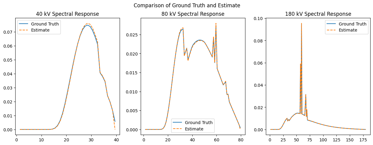
B07. Result Analysis¶

[36]:

import torch
# Get the estimated effective response for each source voltage.
# Make sure to convert to numpy array from tensor before plotting.
est_sp = Estimator.get_spectra()

fig, axs = plt.subplots(1, 3, figsize=(15, 5))

for i in range(3):
    ax = axs[i]
    with torch.no_grad():
        ax.plot(energies[:voltage_list[i]-1], (gt_spec_list[i]/np.trapezoid(gt_spec_list[i],energies))[:voltage_list[i]-1],
                label='Ground Truth')
        es = est_sp[i].numpy()
        es /= np.trapezoid(es,energies)
        ax.plot(energies[:voltage_list[i]-1], es[:voltage_list[i]-1], '--', label='Estimate')

    ax.legend()
    ax.set_title(f'{voltage_list[i]} kV Spectral Response')

fig.suptitle('Comparison of Ground Truth and Estimate')
plt.show()

../_images/examples_T01_Calibration_LEAP_55_0.png

[37]:

import pandas as pd
import torch

# Return a dictionary containing the estimated parameters.
res_params = Estimator.get_params()

# Ground Truth values
ground_truth = {
    "takeoff_angle (degree)": takeoff_angle,
    "fltr_mat": fltr_mat,
    "fltr_th (mm)": fltr_th,
    "det_mat": det_mat,
    "det_th (mm)": det_th,
}

# Estimated values from res_params
# .item() to return value for an estiamted continous parameter.
# material with .formula is because the class Material contains both formula and density.
estimated = {
    "takeoff_angle (degree)": res_params['Reflection_Source_takeoff_angle'].item(),
    "fltr_mat": res_params['Filter_2_material'].formula,
    "fltr_th (mm)": res_params['Filter_2_thickness'].item(),
    "det_mat": res_params['Scintillator_2_material'].formula,
    "det_th (mm)": res_params['Scintillator_2_thickness'].item(),
}

# Combine into a DataFrame for comparison
df = pd.DataFrame({'Ground Truth': ground_truth, 'Estimated': estimated})

# Display the DataFrame
df

[37]:

	Ground Truth	Estimated
takeoff_angle (degree)	13	14.694992
fltr_mat	Al	Al
fltr_th (mm)	3	3.106396
det_mat	CsI	CsI
det_th (mm)	0.33	0.346599