Tutorial 04: Implementing an analytical module for an X-ray component to allow gradient descent
What You Will Need
Parameters: \(a, b, c, \dots\) to be estimated or optimized.
An analtyical model: \(S(E; a, b, c, \dots)\) that defines the spectrum or energy response.
What You Will Expect
How to build an analtyical model?
Implementing the model using PyTorch for differentiability.
A step-by-step guide to setting up and testing the interpolation module.
A. Analytical Model of Filter
A1. Background
In X-ray systems, filters are always used to protect the detector and enhance image quality by selectively absorbing low-energy X-rays that contribute to image noise without improving image contrast. According to Beer’s law, the response of a single filter is
where:
\(m\) denotes the filter material, which is a discrete parameter with only a limited set of choices.
\(\mu(E, m)\) is the Linear Attenuation Coefficient (LAC) of material \(m\) at energy \(E\).
\(\theta\) denotes filter thickness, which is a continuous parameter within a continuous range.
A2. Step-by-Step Implementation
To build an analytical model that supports gradient descent, we need two key functions:
``__init__`` (Initialize the Model)
Defines materials and thickness as model parameters.
Assigns separate memory for continuous parameters corresponding to each discrete material selection.
Enables search over all material combinations, allowing the model to explore different discrete parameter configurations.
``forward`` (Compute Filter Response)
Retrieves the current material and thickness for the filter.
Calls
gen_fltr_res()to compute the X-ray attenuation response using Beer’s Law.Ensures the response is computed for a given set of X-ray energies.
This setup enables efficient spectral modeling and optimization using PyTorch.
The Material class stores the chemical formula and density of a material, ensuring valid input types and allowing it to be used in X-ray modeling and optimization.
The get_lin_att_c_vs_E function calculates the linear attenuation coefficient (LAC) value with density, thickness, and energy vector.
The get_params() function, defined in Base_Spec_Model, retrieves the estimated parameters as a dictionary, applying denormalization and clamping to ensure they remain within valid bounds while maintaining gradient flow for optimization.
[1]:
import numpy as np
import torch
from xcal.models import Base_Spec_Model
from xcal.defs import Material
from xcal.chem_consts._consts_from_table import get_lin_att_c_vs_E

# Implement the analytical model for filter.
def _obtain_attenuation(energies, formula, density, thickness, torch_mode=False):
    # thickness is mm
    mu = get_lin_att_c_vs_E(density, formula, energies)
    if torch_mode:
            mu = torch.tensor(mu)
            att = torch.exp(-mu * thickness)
    else:
            att = np.exp(-mu * thickness)
    return att

def gen_fltr_res(energies, fltr_mat:Material, fltr_th:float, torch_mode=True):

    return _obtain_attenuation(energies, fltr_mat.formula, fltr_mat.density, fltr_th, torch_mode)

# Gradient descent module.
class Filter(Base_Spec_Model):
    def __init__(self, materials, thickness):
        """
        A template filter model based on Beer's Law and NIST mass attenuation coefficients, including all necessary methods.

        Args:
            materials (list): A list of possible materials for the filter,
                where each material should be an instance containing formula and density.
            thickness (tuple or list): If a tuple, it should be (initial value, lower bound, upper bound) for the filter thickness.
                If a list, it should have the same length as the materials list, specifying thickness for each material.
                These values cannot be all None. It will not be optimized when lower == upper.
        """
        if isinstance(thickness, tuple):
            if all(t is None for t in thickness):
                raise ValueError("Thickness tuple cannot have all None values.")
            params_list = [{'material': mat, 'thickness': thickness} for mat in materials]
        elif isinstance(thickness, list):
            if len(thickness) != len(materials):
                raise ValueError("Length of thickness list must match length of materials list.")
            params_list = [{'material': mat, 'thickness': th} for mat, th in zip(materials, thickness)]
        else:
            raise TypeError("Thickness must be either a tuple or a list.")

        super().__init__(params_list)

    def forward(self, energies):
        """
        Takes X-ray energies and returns the filter response.

        Args:
            energies (torch.Tensor): A tensor containing the X-ray energies of a poly-energetic source in units of keV.

        Returns:
            torch.Tensor: The filter response as a function of input energies, selected material, and its thickness.
        """
            # Retrieves
        mat = self.get_params()[f"{self.prefix}_material"]
        th = self.get_params()[f"{self.prefix}_thickness"]
        energies = torch.tensor(energies, dtype=torch.float32) if not isinstance(energies, torch.Tensor) else energies
        return gen_fltr_res(energies, mat, th)
[2]:
import matplotlib.pyplot as plt
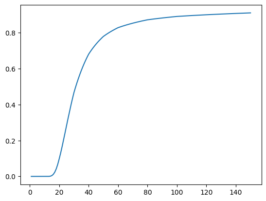
gt_fltr_th = 2.5 # target thickness in um
psb_fltr_mat = [Material(formula='Al', density=2.702), Material(formula='Cu', density=8.92)]
filter_1 = Filter(psb_fltr_mat, thickness=(gt_fltr_th, 0, 10))
ee = np.linspace(1,150,150)
ff = filter_1(ee)
est_param = filter_1.get_params()
print(f'{est_param}')
plt.plot(ee, ff.data)
{'Filter_1_material': Material(formula='Al', density=2.702), 'Filter_1_thickness': tensor(2.5000, grad_fn=<ClampFunctionBackward>)}
[2]:
[<matplotlib.lines.Line2D at 0x15ee0fb50>]
B. An Example of Estimating Filter Thickness
[3]:
max_simkV = 50 # keV
takeoff_angle = 13 # degree
mas_list = 0.01 # Milliampere-seconds

fltr_mat = 'Al' # filter material
fltr_th = 3 # filter thickness in mm

det_mat = 'CsI' # scintillator material
det_density = 4.51 # scintillator density g/cm^3
det_th = 0.33 # scintillator thickness in mm

sample_mats = ['V', 'Al', 'Ti', 'Mg']

ct_info = {
    "SDD": 15,
    "psize": [0.01, 0.01],  # Width and height in mm
}
[4]:
from xcal import get_filter_response,get_scintillator_response
from xcal.chem_consts._periodictabledata import density
import spekpy as sp

simkV = 50
gt_takeoff_angle = 13
s = sp.Spek(kvp=simkV, th=gt_takeoff_angle, dk=1, z=ct_info['SDD']/10, mas=mas_list, char=True)
k, phi_k = s.get_spectrum(edges=False)
phi_k = phi_k * ((ct_info['psize'][0] / 10) * (ct_info['psize'][1] / 10))  #
src_spec = np.zeros(max_simkV-1)
src_spec[:simkV-1] = phi_k  # Assign spectrum values starting from 1.5 keV

ee = k
gt_src = src_spec
gt_fltr = get_filter_response(ee, fltr_mat, density[fltr_mat], fltr_th)
gt_det = get_scintillator_response(ee, det_mat, det_density, det_th)
[5]:
import matplotlib.pyplot as plt
# Plot setup
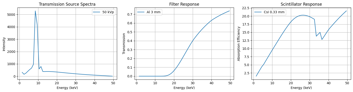
fig, axes = plt.subplots(1, 3, figsize=(15, 4))
# Subplot 1: Source spectra for different voltages
axes[0].plot(ee, src_spec, label=f'{simkV} kVp')
axes[0].set_title('Transmission Source Spectra')
axes[0].set_xlabel('Energy (keV)')
axes[0].set_ylabel('Intensity')
axes[0].legend()
axes[0].grid(True)
# Subplot 2: Filter response
axes[1].plot(ee, gt_fltr, label=f'{fltr_mat} {fltr_th} mm')
axes[1].set_title('Filter Response')
axes[1].set_xlabel('Energy (keV)')
axes[1].set_ylabel('Transmission')
axes[1].legend()
axes[1].grid(True)
# Subplot 3: Scintillator response
axes[2].plot(ee, gt_det, label=f'{det_mat} {det_th} mm')
axes[2].set_title('Scintillator Response')
axes[2].set_xlabel('Energy (keV)')
axes[2].set_ylabel('Absorption Efficiency')
axes[2].legend()
axes[2].grid(True)
# Layout adjustment
plt.tight_layout()
plt.show()
[6]:
import matplotlib.pyplot as plt
import numpy as np
# Assuming ee, gt_srcs, gt_fltr, gt_det, and vol_list are already defined
# Create a new figure with a specified size
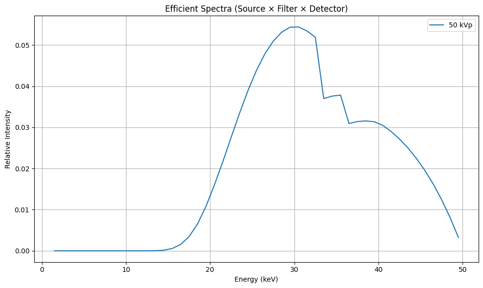
plt.figure(figsize=(10, 6))
gt_spec_list = []
# Plot the efficient spectra for each voltage
# Calculate the efficient spectrum by multiplying with filter and detector responses.
# Then do normalization.
efficient_spectrum = gt_src * gt_fltr * gt_det
gt_spec_list.append(efficient_spectrum)
# efficient_spectrum/=np.trapezoid(efficient_spectrum)
# Plot the efficient spectrum
plt.plot(ee, efficient_spectrum/np.trapezoid(efficient_spectrum), label=f'{simkV} kVp')
# Add labels and title
plt.xlabel('Energy (keV)')
plt.ylabel('Relative Intensity')
plt.title('Efficient Spectra (Source × Filter × Detector)')
plt.legend()
plt.grid(True)
plt.tight_layout()
plt.show()
[7]:
from xcal.chem_consts import get_lin_att_c_vs_E
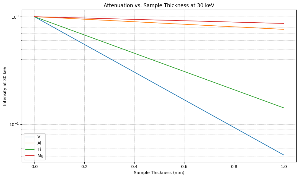
sample_mats = ['V', 'Al', 'Ti', 'Mg']
mat_density = [density[formula] for formula in sample_mats]
lac_vs_E_list = [get_lin_att_c_vs_E(den, formula, ee) for den, formula in zip(mat_density, sample_mats)]
sample_thicknesses = np.linspace(0, 1, 100) # mm
# Attenuation Matrix, multiply effective spectrum can obtain tranmission measurement.
# (4*100)*145: 4 materials, 100 different thicknesses, at total 400 measurements and 145 energy bins.
spec_F = np.concatenate([np.exp(-sample_thicknesses[:,np.newaxis]@lac_vs_E[np.newaxis]) for lac_vs_E in lac_vs_E_list],axis=0)
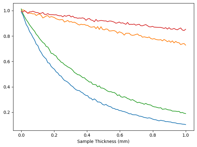
[8]:
import matplotlib.pyplot as plt

# Create a new figure with a specified size
plt.figure(figsize=(10, 6))

# Plot the data for each sample material
for smid, sample_mat in enumerate(sample_mats):
    plt.plot(sample_thicknesses, spec_F[100*smid:100*(smid+1), 30], label=sample_mat)

# Set the y-axis to a logarithmic scale
plt.yscale('log')

# Add labels and title
plt.xlabel('Sample Thickness (mm)')
plt.ylabel('Intensity at 30 keV')
plt.title('Attenuation vs. Sample Thickness at 30 keV')
plt.legend()
plt.grid(True, which='both', linestyle='--', linewidth=0.5)
plt.tight_layout()
plt.show()
[9]:
trans_list = []

# Obtain the converted energy, which is proportional to the detected visible light photons by the camera.
# gt_spec is the converted energy without an object.
# Notice that, trapezoid does the energy integration.
trans = np.trapezoid(spec_F * efficient_spectrum, ee, axis=-1) # Object scan
trans_0 = np.trapezoid(efficient_spectrum, ee, axis=-1) # Air scan value
# Add poisson noise.
# The noise level can be adjusted by changing the mas, the current-time product in the beginning of this tutorial.
trans_noise = np.random.poisson(trans).astype(np.float32)
trans_noise /= trans_0

# Store noisy transmission data.
trans_list.append(trans_noise)
[10]:
import matplotlib.pyplot as plt
import numpy as np

# Determine the number of cases
num_cases = len(gt_spec_list)

# Ensure axes is iterable
if num_cases == 1:
    axes = [axes]

# Plot data for each case

for smid, sample_mat in enumerate(sample_mats):
    # Extract the transmission data for the current sample and case
    transmission_data = trans_list[0][100 * smid : 100 * (smid + 1)]
    plt.plot(sample_thicknesses, transmission_data, label=sample_mat)


# Set the x-axis label for the bottom subplot
plt.xlabel('Sample Thickness (mm)')

# Adjust layout to prevent overlap
plt.tight_layout()
plt.show()
[11]:
from xcal.models import Reflection_Source, Scintillator
from xcal.defs import Material
from xcal.estimate import Estimate
from T04 import Filter

learning_rate = 0.001 # 0.01 for NNAT_LBFGS and 0.001 for Adam
max_iterations = 5000 # 5000 ~ 10000 would be enough
stop_threshold = 1e-6
optimizer_type = 'Adam' # Can also use Adam.

# Use Spekpy to generate a source spectra dictionary.
takeoff_angles = np.linspace(5,45,11)
src_spec_list = []

for ta in takeoff_angles:
    # Generate the X-ray spectrum model with Spekpy for each voltage.
    s = sp.Spek(kvp=simkV, th=ta, dk=1, z=ct_info['SDD'], mas=mas_list, char=True)
    k, phi_k = s.get_spectrum(edges=False)  # Retrieve energy bins and fluence spectrum [Photons cm^-2 keV^-1]

    # Adjust the fluence for the detector pixel area.
    phi_k = phi_k * ((ct_info['psize'][0] / 10) * (ct_info['psize'][1] / 10))  # Convert pixel size from mm² to cm²

    # Initialize a zero-filled spectrum array with length max_simkV.
    src_spec = np.zeros(max_simkV-1)
    src_spec[:simkV-1] = phi_k  # Assign spectrum values starting from 1.5 keV

    # Add the processed spectrum for this voltage to the list.
    src_spec_list.append(src_spec)

src_spec_list = np.array(src_spec_list)
src_spec_list = src_spec_list.reshape((1,len(takeoff_angles),-1))
source = Reflection_Source(voltage=(50, None, None), takeoff_angle=(gt_takeoff_angle, None, None), single_takeoff_angle=True)
source.set_src_spec_list(ee, src_spec_list, [50], takeoff_angles)


# Not estimate filter and scintillator
psb_fltr_mat = [Material(formula='Al', density=2.702),
                Material(formula='Cu', density=8.92)]
filter_1 = Filter(psb_fltr_mat, thickness=(5, 0, 10))
psb_scint_mat = [Material(formula='CsI', density=4.51)]
scintillator_1 = Scintillator(materials=psb_scint_mat, thickness=(0.33, None, None))

spec_models = [[source, filter_1, scintillator_1]]

Estimator = Estimate(ee)
# For each scan, add data and calculated forward matrix to Estimator.
Estimator.add_data(trans_list[0], spec_F, spec_models[0], weight=None)

# Fit data
Estimator.fit(learning_rate=learning_rate,
              max_iterations=max_iterations,
              stop_threshold=stop_threshold,
              optimizer_type=optimizer_type,
              loss_type='transmission',
              logpath=None,
              num_processes=1) # Parallel computing for multiple cpus.
Number of cases for different discrete parameters: 2
2025-05-25 12:51:53,737  - Start Estimation.
2025-05-25 12:51:53,759  - Initial cost: 2.388144e-03
2025-05-25 12:51:53,842  - Iteration: 50
2025-05-25 12:51:53,844  - Cost: 0.0015051235677674413
2025-05-25 12:51:53,844  - Filter_1_material: Material(formula='Al', density=2.702)
2025-05-25 12:51:53,844  - Filter_1_thickness: 4.509207248687744
2025-05-25 12:51:53,845  - Reflection_Source_1_voltage: 50.0
2025-05-25 12:51:53,845  - Reflection_Source_takeoff_angle: 13.0
2025-05-25 12:51:53,845  - Scintillator_2_material: Material(formula='CsI', density=4.51)
2025-05-25 12:51:53,845  - Scintillator_2_thickness: 0.33000001311302185
2025-05-25 12:51:53,845  -
2025-05-25 12:51:53,936  - Iteration: 100
2025-05-25 12:51:53,938  - Cost: 0.0008214872796088457
2025-05-25 12:51:53,938  - Filter_1_material: Material(formula='Al', density=2.702)
2025-05-25 12:51:53,938  - Filter_1_thickness: 4.061138153076172
2025-05-25 12:51:53,938  - Reflection_Source_1_voltage: 50.0
2025-05-25 12:51:53,938  - Reflection_Source_takeoff_angle: 13.0
2025-05-25 12:51:53,938  - Scintillator_2_material: Material(formula='CsI', density=4.51)
2025-05-25 12:51:53,938  - Scintillator_2_thickness: 0.33000001311302185
2025-05-25 12:51:53,938  -
2025-05-25 12:51:54,028  - Iteration: 150
2025-05-25 12:51:54,029  - Cost: 0.00037792042712680995
2025-05-25 12:51:54,030  - Filter_1_material: Material(formula='Al', density=2.702)
2025-05-25 12:51:54,030  - Filter_1_thickness: 3.6804146766662598
2025-05-25 12:51:54,030  - Reflection_Source_1_voltage: 50.0
2025-05-25 12:51:54,030  - Reflection_Source_takeoff_angle: 13.0
2025-05-25 12:51:54,030  - Scintillator_2_material: Material(formula='CsI', density=4.51)
2025-05-25 12:51:54,030  - Scintillator_2_thickness: 0.33000001311302185
2025-05-25 12:51:54,030  -
2025-05-25 12:51:54,109  - Iteration: 200
2025-05-25 12:51:54,111  - Cost: 0.00014460438978858292
2025-05-25 12:51:54,111  - Filter_1_material: Material(formula='Al', density=2.702)
2025-05-25 12:51:54,111  - Filter_1_thickness: 3.387305974960327
2025-05-25 12:51:54,111  - Reflection_Source_1_voltage: 50.0
2025-05-25 12:51:54,111  - Reflection_Source_takeoff_angle: 13.0
2025-05-25 12:51:54,111  - Scintillator_2_material: Material(formula='CsI', density=4.51)
2025-05-25 12:51:54,111  - Scintillator_2_thickness: 0.33000001311302185
2025-05-25 12:51:54,111  -
2025-05-25 12:51:54,212  - Iteration: 250
2025-05-25 12:51:54,214  - Cost: 5.164837057236582e-05
2025-05-25 12:51:54,214  - Filter_1_material: Material(formula='Al', density=2.702)
2025-05-25 12:51:54,214  - Filter_1_thickness: 3.190600633621216
2025-05-25 12:51:54,214  - Reflection_Source_1_voltage: 50.0
2025-05-25 12:51:54,214  - Reflection_Source_takeoff_angle: 13.0
2025-05-25 12:51:54,214  - Scintillator_2_material: Material(formula='CsI', density=4.51)
2025-05-25 12:51:54,214  - Scintillator_2_thickness: 0.33000001311302185
2025-05-25 12:51:54,214  -
2025-05-25 12:51:54,315  - Iteration: 300
2025-05-25 12:51:54,316  - Cost: 2.4953735191957094e-05
2025-05-25 12:51:54,316  - Filter_1_material: Material(formula='Al', density=2.702)
2025-05-25 12:51:54,316  - Filter_1_thickness: 3.0789196491241455
2025-05-25 12:51:54,316  - Reflection_Source_1_voltage: 50.0
2025-05-25 12:51:54,316  - Reflection_Source_takeoff_angle: 13.0
2025-05-25 12:51:54,316  - Scintillator_2_material: Material(formula='CsI', density=4.51)
2025-05-25 12:51:54,316  - Scintillator_2_thickness: 0.33000001311302185
2025-05-25 12:51:54,316  -
2025-05-25 12:51:54,397  - Iteration: 350
2025-05-25 12:51:54,400  - Cost: 1.9495602828101255e-05
2025-05-25 12:51:54,400  - Filter_1_material: Material(formula='Al', density=2.702)
2025-05-25 12:51:54,400  - Filter_1_thickness: 3.025747776031494
2025-05-25 12:51:54,400  - Reflection_Source_1_voltage: 50.0
2025-05-25 12:51:54,400  - Reflection_Source_takeoff_angle: 13.0
2025-05-25 12:51:54,400  - Scintillator_2_material: Material(formula='CsI', density=4.51)
2025-05-25 12:51:54,400  - Scintillator_2_thickness: 0.33000001311302185
2025-05-25 12:51:54,400  -
2025-05-25 12:51:54,470  - Iteration: 400
2025-05-25 12:51:54,472  - Cost: 1.868593790277373e-05
2025-05-25 12:51:54,472  - Filter_1_material: Material(formula='Al', density=2.702)
2025-05-25 12:51:54,472  - Filter_1_thickness: 3.004319429397583
2025-05-25 12:51:54,472  - Reflection_Source_1_voltage: 50.0
2025-05-25 12:51:54,472  - Reflection_Source_takeoff_angle: 13.0
2025-05-25 12:51:54,472  - Scintillator_2_material: Material(formula='CsI', density=4.51)
2025-05-25 12:51:54,472  - Scintillator_2_thickness: 0.33000001311302185
2025-05-25 12:51:54,472  -
2025-05-25 12:51:54,545  - Iteration: 450
2025-05-25 12:51:54,547  - Cost: 1.8596598238218576e-05
2025-05-25 12:51:54,547  - Filter_1_material: Material(formula='Al', density=2.702)
2025-05-25 12:51:54,547  - Filter_1_thickness: 2.9969093799591064
2025-05-25 12:51:54,547  - Reflection_Source_1_voltage: 50.0
2025-05-25 12:51:54,547  - Reflection_Source_takeoff_angle: 13.0
2025-05-25 12:51:54,547  - Scintillator_2_material: Material(formula='CsI', density=4.51)
2025-05-25 12:51:54,547  - Scintillator_2_thickness: 0.33000001311302185
2025-05-25 12:51:54,547  -
2025-05-25 12:51:54,614  - Iteration: 500
2025-05-25 12:51:54,616  - Cost: 1.8589174942462705e-05
2025-05-25 12:51:54,616  - Filter_1_material: Material(formula='Al', density=2.702)
2025-05-25 12:51:54,616  - Filter_1_thickness: 2.9946932792663574
2025-05-25 12:51:54,616  - Reflection_Source_1_voltage: 50.0
2025-05-25 12:51:54,616  - Reflection_Source_takeoff_angle: 13.0
2025-05-25 12:51:54,616  - Scintillator_2_material: Material(formula='CsI', density=4.51)
2025-05-25 12:51:54,616  - Scintillator_2_thickness: 0.33000001311302185
2025-05-25 12:51:54,616  -
2025-05-25 12:51:54,657  - Stopping at epoch 528 because updates are too small.
2025-05-25 12:51:54,657  - Cost: 1.858877294580452e-05
2025-05-25 12:51:54,657  - Filter_1_material: Material(formula='Al', density=2.702)
2025-05-25 12:51:54,657  - Filter_1_thickness: 2.9942777156829834
2025-05-25 12:51:54,657  - Reflection_Source_1_voltage: 50.0
2025-05-25 12:51:54,657  - Reflection_Source_takeoff_angle: 13.0
2025-05-25 12:51:54,657  - Scintillator_2_material: Material(formula='CsI', density=4.51)
2025-05-25 12:51:54,657  - Scintillator_2_thickness: 0.33000001311302185
2025-05-25 12:51:54,657  -
2025-05-25 12:51:54,659  - Start Estimation.
2025-05-25 12:51:54,662  - Initial cost: 9.644821e-02
2025-05-25 12:51:54,731  - Iteration: 50
2025-05-25 12:51:54,733  - Cost: 0.09464140981435776
2025-05-25 12:51:54,733  - Filter_1_material: Material(formula='Cu', density=8.92)
2025-05-25 12:51:54,733  - Filter_1_thickness: 4.4902663230896
2025-05-25 12:51:54,733  - Reflection_Source_1_voltage: 50.0
2025-05-25 12:51:54,733  - Reflection_Source_takeoff_angle: 13.0
2025-05-25 12:51:54,733  - Scintillator_2_material: Material(formula='CsI', density=4.51)
2025-05-25 12:51:54,733  - Scintillator_2_thickness: 0.33000001311302185
2025-05-25 12:51:54,733  -
2025-05-25 12:51:54,802  - Iteration: 100
2025-05-25 12:51:54,804  - Cost: 0.09225913137197495
2025-05-25 12:51:54,804  - Filter_1_material: Material(formula='Cu', density=8.92)
2025-05-25 12:51:54,804  - Filter_1_thickness: 3.9403140544891357
2025-05-25 12:51:54,804  - Reflection_Source_1_voltage: 50.0
2025-05-25 12:51:54,804  - Reflection_Source_takeoff_angle: 13.0
2025-05-25 12:51:54,804  - Scintillator_2_material: Material(formula='CsI', density=4.51)
2025-05-25 12:51:54,804  - Scintillator_2_thickness: 0.33000001311302185
2025-05-25 12:51:54,804  -
2025-05-25 12:51:54,877  - Iteration: 150
2025-05-25 12:51:54,879  - Cost: 0.08896404504776001
2025-05-25 12:51:54,879  - Filter_1_material: Material(formula='Cu', density=8.92)
2025-05-25 12:51:54,879  - Filter_1_thickness: 3.3324739933013916
2025-05-25 12:51:54,879  - Reflection_Source_1_voltage: 50.0
2025-05-25 12:51:54,879  - Reflection_Source_takeoff_angle: 13.0
2025-05-25 12:51:54,879  - Scintillator_2_material: Material(formula='CsI', density=4.51)
2025-05-25 12:51:54,879  - Scintillator_2_thickness: 0.33000001311302185
2025-05-25 12:51:54,879  -
2025-05-25 12:51:54,954  - Iteration: 200
2025-05-25 12:51:54,956  - Cost: 0.08397167176008224
2025-05-25 12:51:54,956  - Filter_1_material: Material(formula='Cu', density=8.92)
2025-05-25 12:51:54,956  - Filter_1_thickness: 2.643720865249634
2025-05-25 12:51:54,956  - Reflection_Source_1_voltage: 50.0
2025-05-25 12:51:54,956  - Reflection_Source_takeoff_angle: 13.0
2025-05-25 12:51:54,956  - Scintillator_2_material: Material(formula='CsI', density=4.51)
2025-05-25 12:51:54,956  - Scintillator_2_thickness: 0.33000001311302185
2025-05-25 12:51:54,956  -
2025-05-25 12:51:55,028  - Iteration: 250
2025-05-25 12:51:55,030  - Cost: 0.07504528015851974
2025-05-25 12:51:55,030  - Filter_1_material: Material(formula='Cu', density=8.92)
2025-05-25 12:51:55,030  - Filter_1_thickness: 1.82919442653656
2025-05-25 12:51:55,030  - Reflection_Source_1_voltage: 50.0
2025-05-25 12:51:55,030  - Reflection_Source_takeoff_angle: 13.0
2025-05-25 12:51:55,030  - Scintillator_2_material: Material(formula='CsI', density=4.51)
2025-05-25 12:51:55,030  - Scintillator_2_thickness: 0.33000001311302185
2025-05-25 12:51:55,030  -
2025-05-25 12:51:55,098  - Iteration: 300
2025-05-25 12:51:55,100  - Cost: 0.04900381714105606
2025-05-25 12:51:55,100  - Filter_1_material: Material(formula='Cu', density=8.92)
2025-05-25 12:51:55,100  - Filter_1_thickness: 0.7538713216781616
2025-05-25 12:51:55,100  - Reflection_Source_1_voltage: 50.0
2025-05-25 12:51:55,100  - Reflection_Source_takeoff_angle: 13.0
2025-05-25 12:51:55,100  - Scintillator_2_material: Material(formula='CsI', density=4.51)
2025-05-25 12:51:55,100  - Scintillator_2_thickness: 0.33000001311302185
2025-05-25 12:51:55,100  -
2025-05-25 12:51:55,171  - Iteration: 350
2025-05-25 12:51:55,173  - Cost: 0.0006778572569601238
2025-05-25 12:51:55,173  - Filter_1_material: Material(formula='Cu', density=8.92)
2025-05-25 12:51:55,173  - Filter_1_thickness: 0.08765144646167755
2025-05-25 12:51:55,173  - Reflection_Source_1_voltage: 50.0
2025-05-25 12:51:55,173  - Reflection_Source_takeoff_angle: 13.0
2025-05-25 12:51:55,173  - Scintillator_2_material: Material(formula='CsI', density=4.51)
2025-05-25 12:51:55,173  - Scintillator_2_thickness: 0.33000001311302185
2025-05-25 12:51:55,173  -
2025-05-25 12:51:55,260  - Iteration: 400
2025-05-25 12:51:55,262  - Cost: 0.00014357846521306783
2025-05-25 12:51:55,262  - Filter_1_material: Material(formula='Cu', density=8.92)
2025-05-25 12:51:55,262  - Filter_1_thickness: 0.10207980126142502
2025-05-25 12:51:55,262  - Reflection_Source_1_voltage: 50.0
2025-05-25 12:51:55,262  - Reflection_Source_takeoff_angle: 13.0
2025-05-25 12:51:55,262  - Scintillator_2_material: Material(formula='CsI', density=4.51)
2025-05-25 12:51:55,262  - Scintillator_2_thickness: 0.33000001311302185
2025-05-25 12:51:55,262  -
2025-05-25 12:51:55,287  - Stopping at epoch 417 because updates are too small.
2025-05-25 12:51:55,287  - Cost: 0.00014372407167684287
2025-05-25 12:51:55,287  - Filter_1_material: Material(formula='Cu', density=8.92)
2025-05-25 12:51:55,287  - Filter_1_thickness: 0.10162963718175888
2025-05-25 12:51:55,287  - Reflection_Source_1_voltage: 50.0
2025-05-25 12:51:55,287  - Reflection_Source_takeoff_angle: 13.0
2025-05-25 12:51:55,287  - Scintillator_2_material: Material(formula='CsI', density=4.51)
2025-05-25 12:51:55,287  - Scintillator_2_thickness: 0.33000001311302185
2025-05-25 12:51:55,287  -
[12]:
Estimator.get_params()
[12]:
{'Reflection_Source_1_voltage': tensor(50.),
 'Reflection_Source_takeoff_angle': tensor(13.),
 'Filter_1_material': Material(formula='Al', density=2.702),
 'Filter_1_thickness': tensor(2.9943, grad_fn=<ClampFunctionBackward>),
 'Scintillator_2_material': Material(formula='CsI', density=4.51),
 'Scintillator_2_thickness': tensor(0.3300)}
[13]:
import torch
# Get the estimated effective response for each source voltage.
# Make sure to convert to numpy array from tensor before plotting.
est_sp = Estimator.get_spectra()

with torch.no_grad():
    plt.plot(ee, (gt_spec_list[0]/np.trapezoid(gt_spec_list[0],ee)),
            label='Ground Truth')
    es = est_sp[0].numpy()
    es /= np.trapezoid(es,ee)
    plt.plot(ee, es, '--', label='Estimate')

plt.legend()
plt.title(f'{simkV} kV Spectral Response')

fig.suptitle('Comparison of Ground Truth and Estimate')
plt.show()
print(f"Ground Truth: {gt_fltr_th:.2f}, Estimated: {Estimator.get_params()['Filter_1_thickness'].item():.2f}")
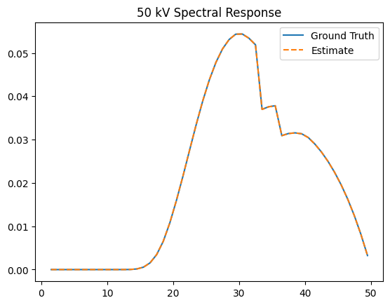
Ground Truth: 2.50, Estimated: 2.99
[13]: