Tutorial 03: Implementing an interpolation module for an X-ray component to allow gradient descent
Introduction
This tutorial covers how to implement an interpolation module for an X-ray component to enable gradient-based optimization. Analytical models are often not reliable for accurately modeling X-ray sources due to complex interactions in the system. Instead, we can use an interpolation model with some lookup tables to achieve a more accurate and flexible representation.
Many physics-based models, such as X-ray source modeling, rely on lookup tables generated using particle simulation tool like Geant4.
We use linear interpolation to create a continuous function based on the lookup table values. This approach ensures that the function is numerically differentiable, allowing for gradient descent optimization.
What You Will Need
User adjustable Parameters: \(v\) is known, like source voltage.
- Estimated Parameters: \(a, b, c, \dots\) to be estimated or optimized.
- An interpolation model: \(S(E, v; a, b, c, \dots)\) that defines the spectrum or energy response.
Lookup table: Precomputed values stored as
\[\mathcal{S}[E, v; i_a, i_b, i_c, \dots]\]where:
\(E\) represents photon energy.
\(v\) represents source voltage.
\(i_a, i_b, i_c, \dots\) are discrete indices for model parameters \(a, b, c, \dots\).
Interpolation: Used to approximate intermediate values between the discrete lookup table entries, ensuring smooth optimization.
What You Will Expect
How to build an interpolation-based model?
Implementing the model using PyTorch for differentiability.
A step-by-step guide to setting up and testing the interpolation module.
A. Interpolation Model of Transmission Source
A1. Background
For a transmission X-ray source, target thickness \(\theta^s\) is essential for the X-ray source spectrum. We want to estimate this parameter. For a given parameter \(\theta^s\) between two discrete points \(\theta_q^s\) and \(\theta_{q+1}^s\), we approximate the function as:
where the interpolation weight \(\gamma\) is given by:
This interpolation provides a smooth approximation of the function and is numerically differentiable, except at the discrete lookup points.
A2. Step-by Step Implementation
To build an interpolation model that supports gradient descent, we need three key functions:
``__init__`` (Initialize the Model)
Defines voltage as adjustable parameter and target thickness as optimizable parameters.
Supports single target thickness for the CT system. If set to true, all instances of this class will use the same target thickness.
``set_src_spec_list`` (Setup Lookup Table & Interpolation)
Loads lookup table data: discrete energies, spectra, voltages, and thicknesses.
Interpolation spectrum over source voltage.
Uses bilinear interpolation (``Interp2D``) to smoothly estimate spectra between discrete points.
``forward`` (Compute Interpolated Spectrum)
Retrieves current model parameters.
Applies 2D interpolation on voltage and target thickness.
Applies 1D interpolation (``Interp1D``) for input energy.
Ensures a continuous, differentiable function for gradient-based optimization.
This setup enables efficient spectral modeling and optimization using PyTorch.
Note 1: Handling Continuous Parameters in Optimization
In the Transmission_Source class, we define voltage and target thickness as optimizable parameters. These parameters are provided as tuples:
``voltage``:
(initial value, lower bound, upper bound)``target_thickness``:
(initial value, lower bound, upper bound)
Key Constraints:
All three values cannot be ``None``, ensuring the parameter is properly defined.
If lower bound == upper bound, the parameter is fixed and will not be optimized.
To handle these parameters, we store them in a dictionary and pass them to the base class:
```python # Build dictionary for continuous parameters params_list = [{‘voltage’: voltage, ‘target_thickness’: target_thickness}] super().__init__(params_list)
Note 2: Handling Data Conversion in ``set_src_spec_list``
In set_src_spec_list, we carefully transition data from lists → NumPy arrays → Torch tensors to ensure compatibility with PyTorch’s function.
[1]:
import numpy as np
import torch
from xcal.models import Base_Spec_Model, prepare_for_interpolation, Interp1D, Interp2D

class Transmission_Source(Base_Spec_Model):
    def __init__(self, voltage, target_thickness, single_target_thickness):
        """
        A template source model designed specifically for reflection sources, including all necessary methods.

        Args:
            voltage (tuple): (initial value, lower bound, upper bound) for the source voltage.
                These three values cannot be all None. It will not be optimized when lower == upper.
            target_thickness (tuple): (initial value, lower bound, upper bound) for the target thickness.
                These three values cannot be all None. It will not be optimized when lower == upper.
            single_target_thickness (bool): If ture, all instances of class transmission source will be the same.

        """
        # Build dictionary for continous parameter.
        params_list = [{'voltage': voltage, 'target_thickness': target_thickness}]
        super().__init__(params_list)

        self.single_target_thickness = single_target_thickness
        if self.single_target_thickness:
            for params in self._params_list:
                params[f"{self.__class__.__name__}_target_thickness"] = params.pop(f"{self.prefix}_target_thickness")
            self._init_estimates()

    def set_src_spec_list(self, energies, src_spec_list, voltages, target_thicknesses):
        """Set source spectra for interpolation, which will be used only by forward function.

        Args:
            src_spec_list (numpy.ndarray): This array contains the reference X-ray source spectra. Each spectrum in this array corresponds to a specific combination of the target_thicknesses and one of the source voltages from src_voltage_list.
            src_voltage_list (numpy.ndarray): This is a sorted array containing the source voltages, each corresponding to a specific reference X-ray source spectrum.
            target_thicknesses (float): This value represents the target_thicknesses, expressed in um, which is used in generating the reference X-ray spectra.
        """
        # Load data
        self.energies = torch.tensor(energies, dtype=torch.float32)
        self.src_spec_list = np.array(src_spec_list)
        self.voltages = np.array(voltages)
        self.target_thicknesses = np.array(target_thicknesses)
        modified_src_spec_list = src_spec_list.copy()

        # Interpolation spectrum over source voltage.
        for tti, tt in enumerate(target_thicknesses):
            modified_src_spec_list[:, tti] = prepare_for_interpolation(modified_src_spec_list[:, tti])

        # Bilinear interpolation
        V, T = torch.meshgrid(torch.tensor(self.voltages, dtype=torch.float32), torch.tensor(self.target_thicknesses, dtype=torch.float32), indexing='ij')
        self.src_spec_interp_func = Interp2D(V, T, torch.tensor(modified_src_spec_list, dtype=torch.float32))

    def forward(self, energies):
        """
        Takes X-ray energies and returns the source spectrum.

        Args:
            energies (torch.Tensor): A tensor containing the X-ray energies of a poly-energetic source in units of keV.

        Returns:
            torch.Tensor: The source response.
        """
        #  Retrieves voltage and target thickness
        voltage = self.get_params()[f"{self.prefix}_voltage"]
        if self.single_target_thickness:
            target_thickness = self.get_params()[f"{self.__class__.__name__}_target_thickness"]
        else:
            target_thickness = self.get_params()[f"{self.prefix}_target_thickness"]

        # Applies 2D interpolation on voltage and target thickness.
        src_spec = self.src_spec_interp_func(voltage, target_thickness)

        # Build 1D interpolation function with src_spec.
        src_interp_E_func = Interp1D(self.energies, src_spec)

        # Applies 1D interpolation function for input energy.
        energies = torch.tensor(energies, dtype=torch.float32) if not isinstance(energies, torch.Tensor) else energies
        return src_interp_E_func(energies)
A3. Usage of Transmission Source
[2]:
import pandas as pd

def integrate_by_step(data, step_size, offset=0):
    num_elements = len(data)

    # Calculate the number of chunks
    num_chunks = (num_elements // step_size) + (1 if num_elements % step_size else 0)

    # Generate the chunks and sum their elements
    integrated_data = [sum(data[i*step_size-offset : (i)*step_size+step_size-offset]) for i in range(num_chunks)]

    return np.array(integrated_data)

psize = 0.01 # mm
max_simkV=150
energies_lookup = np.linspace(1, max_simkV, max_simkV)

# Define the kVp and Wth values for the lookup table
kvp_values = [40, 80, 150]
wth_values = [1, 3, 5, 7]

# Read data from lookup table.
data = []
df = pd.read_csv('./data/lookup_tables/Geant4_Transmission_Source_Spectra.csv', header=[0,1,2,3,4,5])
df.columns.set_names(['W_Thickness', 'Diamond_Thickness', 'Angle', 'PhysicsModel', 'Voltage', 'Energy (keV)'], inplace=True)

# Prepare lookup table data for set_src_spec_list.
for kvp in kvp_values:
    wth_data = []
    for wth in wth_values:
        # Load the data, skipping the first row
        # Specify which spectrum is read from the large csv file based on Target thickness, Apex Angle, Physics Model in Geant4, and Source Voltage.
        csv_data = df.xs(('%dum'%wth,
                          '10deg',
                          'G4EmLivermorePhysics',
                          '%dkVp'%kvp),
                         level=['W_Thickness', 'Angle','PhysicsModel','Voltage'], axis=1)*psize*psize
        # Convert bin size from 0.1 keV to 1 keV.
        sp_integral = integrate_by_step(csv_data.values[9:,0],step_size=10,offset=5)
        # Append only the y-axis data (second column)
        wth_data.append(sp_integral)


    # Stack the Wth data for this particular kVp
    data.append(np.array(wth_data))

# Convert the list to a 3D numpy array
padded_spec_table = np.array(data)
print('Lookup Table has dimension:', padded_spec_table.shape)
print(f'{len(kvp_values)}  source voltages')
print(f'{len(wth_values)}  target thicknesses')
print(f'{len(energies_lookup)}  energy bins')
padded_spec_table = np.pad(padded_spec_table, ((0, 0), (0, 0), (0, 10)), mode='constant', constant_values=0)
Lookup Table has dimension: (3, 4, 150)
3  source voltages
4  target thicknesses
150  energy bins
What will get from this example?
A differentiable function for the transmission source, \(S (E, v; \theta^s)\), which depends on the source voltage and target thickness, and outputs a one-dimensional source spectrum corresponding to the energy vector.
[3]:
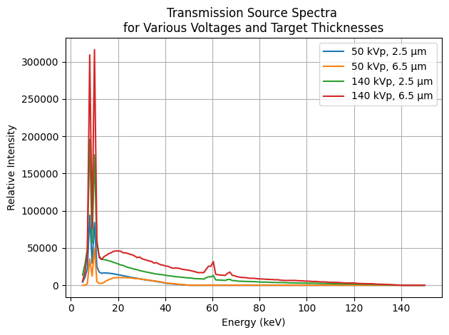
import matplotlib.pyplot as plt
import numpy as np

# Define energy vector for output.
ee = np.linspace(5, 150, 145)

# Define parameter combinations of source voltage (kVp) and tungsten target thickness (μm)
param_combinations = [
    {'voltage': 50, 'thickness': 2.5},
    {'voltage': 50, 'thickness': 6.5},
    {'voltage': 140, 'thickness': 2.5},
    {'voltage': 140, 'thickness': 6.5},
]

# Plot spectra for each combination
for combo in param_combinations:
    v = combo['voltage']
    theta_s = combo['thickness']

    # Initialize the transmission source
    source = Transmission_Source(
        voltage=(v, None, None),
        target_thickness=(theta_s, 1, 7),
        single_target_thickness=True
    )

    # Set the source spectrum list
    source.set_src_spec_list(energies_lookup, padded_spec_table, kvp_values, wth_values)

    # Compute the spectrum
    ss = source(ee)

    # Plot the spectrum with a label
    plt.plot(ee, ss.data, label=f'{v} kVp, {theta_s} μm')

# Customize the plot
plt.xlabel('Energy (keV)')
plt.ylabel('Relative Intensity')
plt.title('Transmission Source Spectra \nfor Various Voltages and Target Thicknesses')
plt.legend()
plt.grid(True)
plt.tight_layout()
plt.show()
B. An Example of Estimating Target Thickness.
B1. Data Simulation
[4]:
from xcal import get_filter_response,get_scintillator_response
from xcal.chem_consts._periodictabledata import density

gt_src_tgt_th = 4.5 # micrometer
vol_list = [40, 80, 150] # kV

fltr_mat = 'Al' # filter material
fltr_th = 3 # filter thickness in mm

det_mat = 'CsI' # scintillator material
det_density = 4.51 # scintillator density g/cm^3
det_th = 0.33 # scintillator thickness in mm

# For generating ground truth, set min and max to None for disable optimization.
src_modules = [Transmission_Source(
        voltage=(v, None, None),
        target_thickness=(gt_src_tgt_th, None, None),
        single_target_thickness=True
    ) for v in vol_list]

[source.set_src_spec_list(energies_lookup, padded_spec_table, kvp_values, wth_values) for source in src_modules]
gt_srcs = [source(ee) for source in src_modules]
gt_fltr = get_filter_response(ee, fltr_mat, density[fltr_mat], fltr_th)
gt_det = get_scintillator_response(ee, det_mat, det_density, det_th)
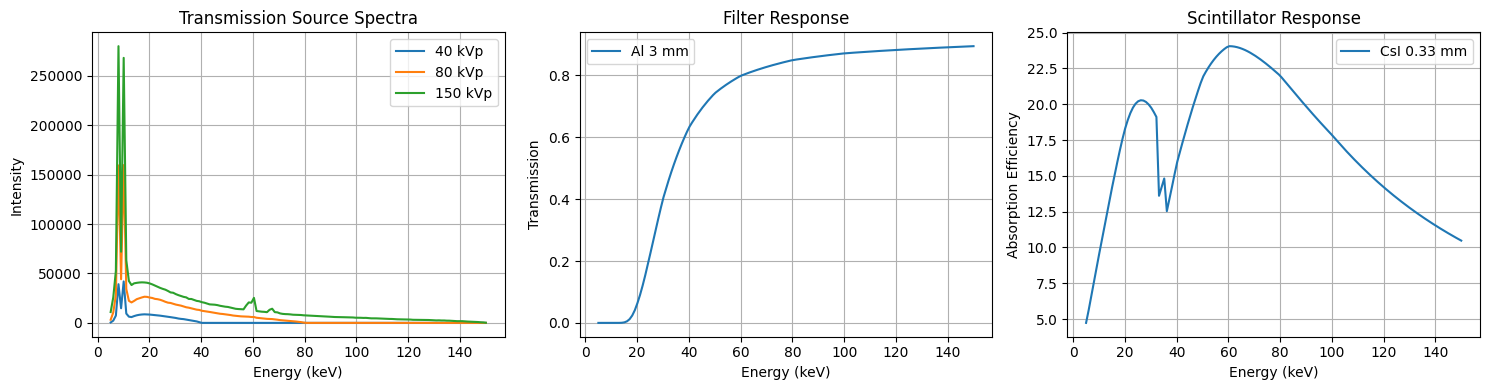
[5]:
import matplotlib.pyplot as plt

# Plot setup
fig, axes = plt.subplots(1, 3, figsize=(15, 4))

# Subplot 1: Source spectra for different voltages
for i, (v, spec) in enumerate(zip(vol_list, gt_srcs)):
    axes[0].plot(ee, spec.data, label=f'{v} kVp')
axes[0].set_title('Transmission Source Spectra')
axes[0].set_xlabel('Energy (keV)')
axes[0].set_ylabel('Intensity')
axes[0].legend()
axes[0].grid(True)

# Subplot 2: Filter response
axes[1].plot(ee, gt_fltr, label=f'{fltr_mat} {fltr_th} mm')
axes[1].set_title('Filter Response')
axes[1].set_xlabel('Energy (keV)')
axes[1].set_ylabel('Transmission')
axes[1].legend()
axes[1].grid(True)

# Subplot 3: Scintillator response
axes[2].plot(ee, gt_det, label=f'{det_mat} {det_th} mm')
axes[2].set_title('Scintillator Response')
axes[2].set_xlabel('Energy (keV)')
axes[2].set_ylabel('Absorption Efficiency')
axes[2].legend()
axes[2].grid(True)

# Layout adjustment
plt.tight_layout()
plt.show()
[6]:
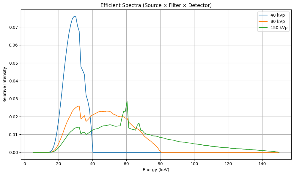
import matplotlib.pyplot as plt
import numpy as np

# Assuming ee, gt_srcs, gt_fltr, gt_det, and vol_list are already defined

# Create a new figure with a specified size
plt.figure(figsize=(10, 6))
gt_spec_list = []
# Plot the efficient spectra for each voltage
for v, spec in zip(vol_list, gt_srcs):
    # Convert spec.data to a NumPy array if it's not already
    spectrum = np.asarray(spec.data)
    # Calculate the efficient spectrum by multiplying with filter and detector responses.
    # Then do normalization.
    efficient_spectrum = spectrum * gt_fltr * gt_det
    gt_spec_list.append(efficient_spectrum)
    # efficient_spectrum/=np.trapezoid(efficient_spectrum)
    # Plot the efficient spectrum
    plt.plot(ee, efficient_spectrum/np.trapezoid(efficient_spectrum), label=f'{v} kVp')

# Add labels and title
plt.xlabel('Energy (keV)')
plt.ylabel('Relative Intensity')
plt.title('Efficient Spectra (Source × Filter × Detector)')
plt.legend()
plt.grid(True)
plt.tight_layout()
plt.show()
[7]:
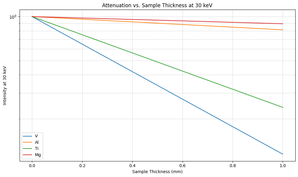
from xcal.chem_consts import get_lin_att_c_vs_E
sample_mats = ['V', 'Al', 'Ti', 'Mg']
mat_density = [density[formula] for formula in sample_mats]
lac_vs_E_list = [get_lin_att_c_vs_E(den, formula, ee) for den, formula in zip(mat_density, sample_mats)]
sample_thicknesses = np.linspace(0, 1, 100) # mm

# Attenuation Matrix, multiply effective spectrum can obtain tranmission measurement.
# (4*100)*145: 4 materials, 100 different thicknesses, at total 400 measurements and 145 energy bins.
spec_F = np.concatenate([np.exp(-sample_thicknesses[:,np.newaxis]@lac_vs_E[np.newaxis]) for lac_vs_E in lac_vs_E_list],axis=0)
[8]:
import matplotlib.pyplot as plt

# Create a new figure with a specified size
plt.figure(figsize=(10, 6))

# Plot the data for each sample material
for smid, sample_mat in enumerate(sample_mats):
    plt.plot(sample_thicknesses, spec_F[100*smid:100*(smid+1), 30], label=sample_mat)

# Set the y-axis to a logarithmic scale
plt.yscale('log')

# Add labels and title
plt.xlabel('Sample Thickness (mm)')
plt.ylabel('Intensity at 30 keV')
plt.title('Attenuation vs. Sample Thickness at 30 keV')
plt.legend()
plt.grid(True, which='both', linestyle='--', linewidth=0.5)
plt.tight_layout()
plt.show()
[9]:
trans_list = []
for case_i, gt_spec in zip(np.arange(len(gt_spec_list)), gt_spec_list):
    # Obtain the converted energy, which is proportional to the detected visible light photons by the camera.
    # gt_spec is the converted energy without an object.
    # Notice that, trapezoid does the energy integration.
    trans = np.trapezoid(spec_F * gt_spec, ee, axis=-1) # Object scan
    trans_0 = np.trapezoid(gt_spec, ee, axis=-1) # Air scan value
    # Add poisson noise.
    # The noise level can be adjusted by changing the mas, the current-time product in the beginning of this tutorial.
    trans_noise = np.random.poisson(trans).astype(np.float32)
    trans_noise /= trans_0

    # Store noisy transmission data.
    trans_list.append(trans_noise)
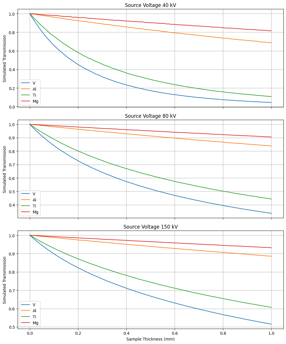
[10]:
import matplotlib.pyplot as plt
import numpy as np

# Determine the number of cases
num_cases = len(gt_spec_list)

# Create subplots: one row per case
fig, axes = plt.subplots(nrows=num_cases, ncols=1, figsize=(10, 4 * num_cases), sharex=True)

# Ensure axes is iterable
if num_cases == 1:
    axes = [axes]

# Plot data for each case
for case_i, (ax, gt_spec) in enumerate(zip(axes, gt_spec_list)):
    for smid, sample_mat in enumerate(sample_mats):
        # Extract the transmission data for the current sample and case
        transmission_data = trans_list[case_i][100 * smid : 100 * (smid + 1)]
        ax.plot(sample_thicknesses, transmission_data, label=sample_mat)

    # Set title and labels for the subplot
    ax.set_title(f'Source Voltage {vol_list[case_i]} kV')
    ax.set_ylabel('Simulated Transmission')
    ax.grid(True)
    ax.legend()

# Set the x-axis label for the bottom subplot
axes[-1].set_xlabel('Sample Thickness (mm)')

# Adjust layout to prevent overlap
plt.tight_layout()
plt.show()
B2. Estimation
[11]:
from xcal.models import  Filter, Scintillator
from xcal.defs import Material
from xcal.estimate import Estimate
from T03 import Transmission_Source

learning_rate = 0.001 # 0.01 for NNAT_LBFGS and 0.001 for Adam
max_iterations = 5000 # 5000 ~ 10000 would be enough
stop_threshold = 1e-6
optimizer_type = 'Adam' # Can also use Adam.

# For optimization, set min and max to reasonable range
sources = [Transmission_Source(
        voltage=(v, None, None),
        target_thickness=(4, 1, 7), # GT is 4.5
        single_target_thickness=True
    ) for v in vol_list]

[source.set_src_spec_list(energies_lookup, padded_spec_table, kvp_values, wth_values) for source in sources]

# Not estimate filter and scintillator
psb_fltr_mat = [Material(formula='Al', density=2.702), ]
filter_1 = Filter(psb_fltr_mat, thickness=(3, None, None))
psb_scint_mat = [Material(formula='CsI', density=4.51)]
scintillator_1 = Scintillator(materials=psb_scint_mat, thickness=(0.33, None, None))

spec_models = [[source, filter_1, scintillator_1] for source in sources]

Estimator = Estimate(ee)
# For each scan, add data and calculated forward matrix to Estimator.
for nrad, concatenate_models in zip(trans_list, spec_models):
    Estimator.add_data(nrad, spec_F, concatenate_models, weight=None)

# Fit data
Estimator.fit(learning_rate=learning_rate,
              max_iterations=max_iterations,
              stop_threshold=stop_threshold,
              optimizer_type=optimizer_type,
              loss_type='transmission',
              logpath=None,
              num_processes=1) # Parallel computing for multiple cpus.
Number of cases for different discrete parameters: 1
2025-05-25 11:47:34,144  - Start Estimation.
2025-05-25 11:47:34,171  - Initial cost: 3.992899e-06
2025-05-25 11:47:34,510  - Iteration: 50
2025-05-25 11:47:34,517  - Cost: 1.749823240970727e-06
2025-05-25 11:47:34,517  - Filter_2_material: Material(formula='Al', density=2.702)
2025-05-25 11:47:34,517  - Filter_2_thickness: 3.0
2025-05-25 11:47:34,517  - Scintillator_2_material: Material(formula='CsI', density=4.51)
2025-05-25 11:47:34,517  - Scintillator_2_thickness: 0.33000001311302185
2025-05-25 11:47:34,517  - Transmission_Source_1_voltage: 40.0
2025-05-25 11:47:34,517  - Transmission_Source_2_voltage: 80.0
2025-05-25 11:47:34,517  - Transmission_Source_3_voltage: 150.0
2025-05-25 11:47:34,517  - Transmission_Source_target_thickness: 4.273849010467529
2025-05-25 11:47:34,517  -
2025-05-25 11:47:34,838  - Iteration: 100
2025-05-25 11:47:34,845  - Cost: 1.1709183809216483e-06
2025-05-25 11:47:34,845  - Filter_2_material: Material(formula='Al', density=2.702)
2025-05-25 11:47:34,845  - Filter_2_thickness: 3.0
2025-05-25 11:47:34,845  - Scintillator_2_material: Material(formula='CsI', density=4.51)
2025-05-25 11:47:34,845  - Scintillator_2_thickness: 0.33000001311302185
2025-05-25 11:47:34,845  - Transmission_Source_1_voltage: 40.0
2025-05-25 11:47:34,845  - Transmission_Source_2_voltage: 80.0
2025-05-25 11:47:34,845  - Transmission_Source_3_voltage: 150.0
2025-05-25 11:47:34,845  - Transmission_Source_target_thickness: 4.436107158660889
2025-05-25 11:47:34,845  -
2025-05-25 11:47:35,173  - Iteration: 150
2025-05-25 11:47:35,179  - Cost: 1.1181043646502076e-06
2025-05-25 11:47:35,180  - Filter_2_material: Material(formula='Al', density=2.702)
2025-05-25 11:47:35,180  - Filter_2_thickness: 3.0
2025-05-25 11:47:35,180  - Scintillator_2_material: Material(formula='CsI', density=4.51)
2025-05-25 11:47:35,180  - Scintillator_2_thickness: 0.33000001311302185
2025-05-25 11:47:35,180  - Transmission_Source_1_voltage: 40.0
2025-05-25 11:47:35,180  - Transmission_Source_2_voltage: 80.0
2025-05-25 11:47:35,180  - Transmission_Source_3_voltage: 150.0
2025-05-25 11:47:35,180  - Transmission_Source_target_thickness: 4.491504669189453
2025-05-25 11:47:35,180  -
2025-05-25 11:47:35,512  - Iteration: 200
2025-05-25 11:47:35,519  - Cost: 1.1168338005518308e-06
2025-05-25 11:47:35,519  - Filter_2_material: Material(formula='Al', density=2.702)
2025-05-25 11:47:35,519  - Filter_2_thickness: 3.0
2025-05-25 11:47:35,519  - Scintillator_2_material: Material(formula='CsI', density=4.51)
2025-05-25 11:47:35,519  - Scintillator_2_thickness: 0.33000001311302185
2025-05-25 11:47:35,519  - Transmission_Source_1_voltage: 40.0
2025-05-25 11:47:35,519  - Transmission_Source_2_voltage: 80.0
2025-05-25 11:47:35,519  - Transmission_Source_3_voltage: 150.0
2025-05-25 11:47:35,519  - Transmission_Source_target_thickness: 4.500911235809326
2025-05-25 11:47:35,519  -
2025-05-25 11:47:35,686  - Stopping at epoch 225 because updates are too small.
2025-05-25 11:47:35,686  - Cost: 1.1168305036335369e-06
2025-05-25 11:47:35,686  - Filter_2_material: Material(formula='Al', density=2.702)
2025-05-25 11:47:35,686  - Filter_2_thickness: 3.0
2025-05-25 11:47:35,686  - Scintillator_2_material: Material(formula='CsI', density=4.51)
2025-05-25 11:47:35,686  - Scintillator_2_thickness: 0.33000001311302185
2025-05-25 11:47:35,686  - Transmission_Source_1_voltage: 40.0
2025-05-25 11:47:35,686  - Transmission_Source_2_voltage: 80.0
2025-05-25 11:47:35,686  - Transmission_Source_3_voltage: 150.0
2025-05-25 11:47:35,686  - Transmission_Source_target_thickness: 4.501378536224365
2025-05-25 11:47:35,686  -
[12]:
import torch
# Get the estimated effective response for each source voltage.
# Make sure to convert to numpy array from tensor before plotting.
est_sp = Estimator.get_spectra()

fig, axs = plt.subplots(1, 3, figsize=(15, 5))

for i in range(3):
    ax = axs[i]
    with torch.no_grad():
        ax.plot(ee, (gt_spec_list[i]/np.trapezoid(gt_spec_list[i],ee)),
                label='Ground Truth')
        es = est_sp[i].numpy()
        es /= np.trapezoid(es,ee)
        ax.plot(ee, es, '--', label='Estimate')

    ax.legend()
    ax.set_title(f'{vol_list[i]} kV Spectral Response')

fig.suptitle('Comparison of Ground Truth and Estimate')
plt.show()
print(f"Ground Truth: {gt_src_tgt_th:.2f}, Estimated: {Estimator.get_params()['Transmission_Source_target_thickness'].item():.2f}")
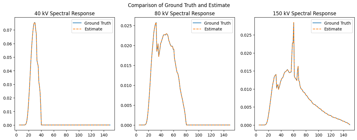
Ground Truth: 4.50, Estimated: 4.50